Grapht: graph connectedness and dimensionality

I’ve been toying around with graph stuff from time to time for a while now.  I still have pretty much no idea what I am doing, but I enjoy having a field to dive into on occasion. As part of that, I’ve been working on a toy project on github for playing with graphs: Grapht

At this stage, all it really does is some basic creation of graphs as sparse adjacency matrices, and some simple calculations on those graphs.  Something I was interested in (for some reason), was the interaction between conntectedness/sparsity and dimension in the adjacency matrices of directed graphs.  So first, a quick overview of what I’m talking about:

Graphs

A graph is a simple data structure that is basically a collection of nodes, connected to each other by edges.  A common type of graph is a social network, so each node is a person, and the edges that connect them are friendships.  This can get complicated by things like edge weightings, and an endless list of mathematical abstractions, but we can think of graphs as just nodes and edges for the sake of this post.

In this simple kind of graph, we have two distinctions: directed and undirected.  To continue using the social network example, a directed graph would mean that Joe can be friends with Beth, while Beth is not friends with Joe.  Undirected means everything is a two way street. So how can we represent this?  Let’s look at a matrix of friendships (we will be optimists and say that the friendships are undirected, so all two-way-streets).

Adjacency Matrix

To look at this case, we will draw out what is referred to as an Adjacency Matrix.

  |Joe Beth Jim Jane

Joe | 0 1 0 1
Beth | 1 0 0 0 Jim | 0 0 0 0 Jane | 1 0 0 0

So every point in the matrix has a 1 if there is a friendship present (Beth-Joe and Joe-Jane).  Immediately we can see a few things:

- The diagonal is always 0

- The matrix is sparse and binary

- The matrix is square

- The matrix is symmetric

So that’s all cool.  What about friends-of-friends?

  |Joe Beth Jim Jane

Joe | 0 1 0 1
Beth | 1 0 0 1 Jim | 0 0 0 0 Jane | 1 1 0 0

Turns out to get the 2nd degree connections of a network, you can just use the sign of the dot product of the adjacency matrices.  In pseudocode:

A_second_connections = sign(A.dot(A))

To get the 3rd degree you just dot multiply with the original adjacency matrix again.  Pretty easy!

A_third_connections = sign(sign(A.dot(A)).dot(A))

The problem

It turns out the adjacency matrix is a pretty convenient way to do things for simple graphs. Exploiting those things we observed about the first matrix (some specific to undirected graphs), we can quickly conclude that:

- The graph can likely be represented efficiently with a sparse matrix (if most people aren't friends with most people)

- If the graph is undirected, we really only need the upper triangle, excluding the diagonal.

- We can simply calculate the N-degree connection equivalent graph

- As N gets big, the matrix will get less sparse.

That last point is really the purpose of this post. It’s a pretty dumb little problem, but I thought it was interesting, so I used Grapht to find out what the relationship between dimensionality (number of people in our network) and N is, when it comes to sparsity of our resultant adjacency matrix.

The code

To do this, we use the DenseGraph interface in Grapht to generate a couple of thousand different (directed) graphs and see what their densities look like at different Ns.  Each graph differs by the dimensionality, or the number of nodes in the graph.

We kept the average number of edges per node approximately constant by setting the density of the initial randomly generated matrix.  We then calculate the density of the initial (zero-hop), two hop, and three hop graphs.

from grapht.graph import DenseGraph import random import numpy as np import pandas as pd import matplotlib.pyplot as plt import matplotlib matplotlib.style.use(‘ggplot’)

output = [] con_per_con = 5

for dim in range(1, 2000): # Make an array density = float(dim * con_per_con) / float(dim * dim) A = np.array([[1 if random.random() < density else 0 for _ in range(dim)] for _ in range(dim)])

# Instantiate the graph
gp = DenseGraph(A)

# Calc the as-is ratio
before_ratio = gp.get_nnz() / float(dim * dim)

# Calc the the 1-hop adj
hop_matrix = gp.get_n_connection(n=2).toarray()
gp2 = DenseGraph(hop_matrix)
after_ratio = gp2.get_nnz() / float(dim * dim)

# Calc the the 2-hop adj
two_hop_matrix = gp.get_n_connection(n=3).toarray()
gp3 = DenseGraph(two_hop_matrix)
two_ratio = gp3.get_nnz() / float(dim * dim)
output.append([before_ratio, after_ratio, two_ratio])
print(dim)

df = pd.DataFrame(output, columns=[‘Zero Hop’, ‘One Hop’, ‘Two Hop’])

ax = df.plot() plt.title(‘Connectedness of Adjacency Matrices Based On Dimension\n(%s connections per node held constant)’ % con_per_con) plt.xlabel(‘Dimension (number of nodes)’) plt.ylabel(‘Connectedness (percentage of non-zero entries)’) plt.show()

The result

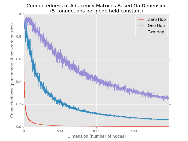
Pretty neat. As you’d expect, the matrices all get generally sparser as the number of nodes increases, but at different rates depending on the number of hops.  Try it out yourself with different average numbers of edges per node, it’s pretty interesting.  I’m not sure where the limit is where a sparse matrix becomes more efficient than a dense one computationally, but I would love to figure that out and have Grapht figure out when to switch automatically for this kind of operation.

Anyway, hopefully you all found this as interesting as I did, let me know here or on Github if you have any ideas or find this useful.

-Will