BinaryEncoder: The Space-Efficient Alternative to One-Hot Encoding
In our previous posts, we explored OneHotEncoder and OrdinalEncoder, two fundamental approaches to handling categorical data. Today, we’ll dive into a clever (or hacky) middle ground: the BinaryEncoder from category_encoders.
Binary encoding attempts to offer a compromise between the dimensionality explosion of one-hot encoding and the potentially problematic ordinality of ordinal encoding. It was one of the experiments from my original blog series on the subject, and while it does acheive the goal of lower resulting dimension than one-hot encoding, it’s not really based on any particular mathematical theory and is more akin to the hashing trick: convinient in some specific cases. Let’s explore how it works and when to use it.
The Problem: Finding the Sweet Spot
One-hot encoding creates a new column for each category, which can lead to a massive increase in dimensionality for high-cardinality features. On the other hand, ordinal encoding is compact but imposes an arbitrary ordering on categories. The use case that inspired this was fault codes, we often saw cardinalities in the 10s of hundreds of thousands with no natural ordering.
Binary encoding offers an elegant solution: it represents each category as its binary code, creating a much more compact representation than one-hot encoding while avoiding some of the drawbacks of ordinal encoding.
How Binary Encoding Works
The process involves three main steps:
- Ordinal encoding: First, each category is assigned a unique integer (just like in ordinal encoding)
- Binary conversion: Each integer is converted to its binary representation
- Bit splitting: Each bit of the binary representation becomes a separate column
For example, with 5 categories:
| Category | Ordinal | Binary | Binary Columns |
|---|---|---|---|
| A | 0 | 000 | 0, 0, 0 |
| B | 1 | 001 | 0, 0, 1 |
| C | 2 | 010 | 0, 1, 0 |
| D | 3 | 011 | 0, 1, 1 |
| E | 4 | 100 | 1, 0, 0 |
Instead of creating 5 columns (as one-hot encoding would), binary encoding creates only 3 columns (log₂(5) rounded up). For large numbers of categories, this difference becomes substantial.
Implementation with category_encoders
The category_encoders library provides an efficient implementation of binary encoding:
import pandas as pd
import category_encoders as ce
import numpy as np
import matplotlib.pyplot as plt
import seaborn as sns

# Sample data
data = pd.DataFrame({
    'color': ['red', 'blue', 'green', 'yellow', 'orange', 'purple', 'red', 'green'],
    'size': ['small', 'medium', 'large', 'medium', 'small', 'large', 'medium', 'small'],
    'price': [10.5, 15.0, 20.0, 18.5, 12.0, 22.5, 11.0, 19.5]
})

# Initialize the encoder
encoder = ce.BinaryEncoder(cols=['color', 'size'])

# Fit and transform
encoded_data = encoder.fit_transform(data)
print(encoded_data)
This produces the following output:
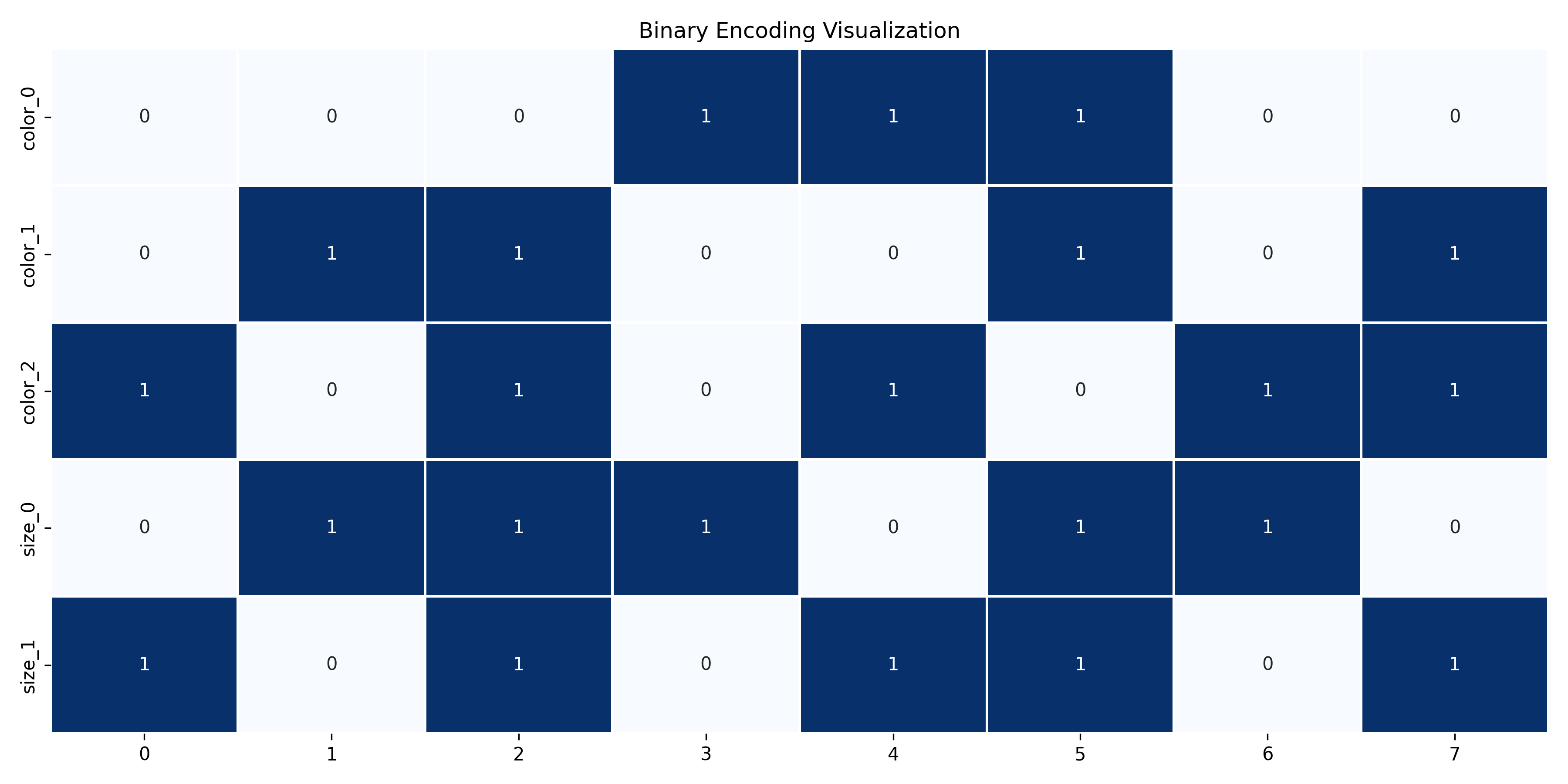
   color_0  color_1  color_2  size_0  size_1  price
0        0        0        1       0       1   10.5
1        0        1        0       1       0   15.0
2        0        1        1       1       1   20.0
3        1        0        0       1       0   18.5
4        1        0        1       0       1   12.0
5        1        1        0       1       1   22.5
6        0        0        1       1       0   11.0
7        0        1        1       0       1   19.5
We can visualize this encoding with a heatmap:
# Visualize the encoding
plt.figure(figsize=(12, 6))
encoded_cols = [col for col in encoded_data.columns if col != 'price']
sns.heatmap(encoded_data[encoded_cols].T, cmap='Blues',
            annot=True, fmt='d', cbar=False, linewidths=1)
plt.title('Binary Encoding Visualization')
plt.tight_layout()
Key Features of category_encoders.BinaryEncoder
The BinaryEncoder in category_encoders offers several useful features:
1. Pandas integration
# Direct support for pandas DataFrames
encoded_df = encoder.fit_transform(df)
2. Column specification by name
# Encode only specific columns by name
encoder = ce.BinaryEncoder(cols=['color', 'size'])
3. Inverse transform
# Convert back to original representation
original_data = encoder.inverse_transform(encoded_data)
Real-World Example: Product Recommendation System
Let’s use BinaryEncoder in a practical scenario - a product recommendation system with high-cardinality categorical features:
import pandas as pd
import category_encoders as ce
import numpy as np
from sklearn.model_selection import train_test_split
from sklearn.ensemble import GradientBoostingRegressor
from sklearn.metrics import mean_squared_error

# Sample product data with high-cardinality categories
np.random.seed(42)
n_samples = 10000

# Generate synthetic data
product_ids = [f'P{i}' for i in range(1000)]  # 1000 unique products
category_ids = [f'C{i}' for i in range(100)]  # 100 unique categories
brand_ids = [f'B{i}' for i in range(50)]      # 50 unique brands

data = pd.DataFrame({
    'product_id': np.random.choice(product_ids, n_samples),
    'category_id': np.random.choice(category_ids, n_samples),
    'brand_id': np.random.choice(brand_ids, n_samples),
    'price': np.random.uniform(10, 1000, n_samples),
    'rating': np.random.uniform(1, 5, n_samples)
})

# Split the data
X = data.drop('rating', axis=1)
y = data['rating']
X_train, X_test, y_train, y_test = train_test_split(X, y, test_size=0.2, random_state=42)

# Compare encoding methods
encoders = {
    'one-hot': ce.OneHotEncoder(cols=['product_id', 'category_id', 'brand_id']),
    'binary': ce.BinaryEncoder(cols=['product_id', 'category_id', 'brand_id']),
    'ordinal': ce.OrdinalEncoder(cols=['product_id', 'category_id', 'brand_id'])
}

results = {}

for name, encoder in encoders.items():
    print(f"Processing {name} encoder...")

    # Encode the data
    X_train_encoded = encoder.fit_transform(X_train)
    X_test_encoded = encoder.transform(X_test)

    # Train a model
    model = GradientBoostingRegressor(n_estimators=100, random_state=42)
    model.fit(X_train_encoded, y_train)

    # Make predictions
    y_pred = model.predict(X_test_encoded)

    # Evaluate
    mse = mean_squared_error(y_test, y_pred)
    results[name] = {
        'MSE': mse,
        'RMSE': np.sqrt(mse),
        'Feature Count': X_train_encoded.shape[1]
    }

# Display results
results_df = pd.DataFrame(results).T
print("\nResults:")
print(results_df)
The results show the trade-off between feature count and model performance:
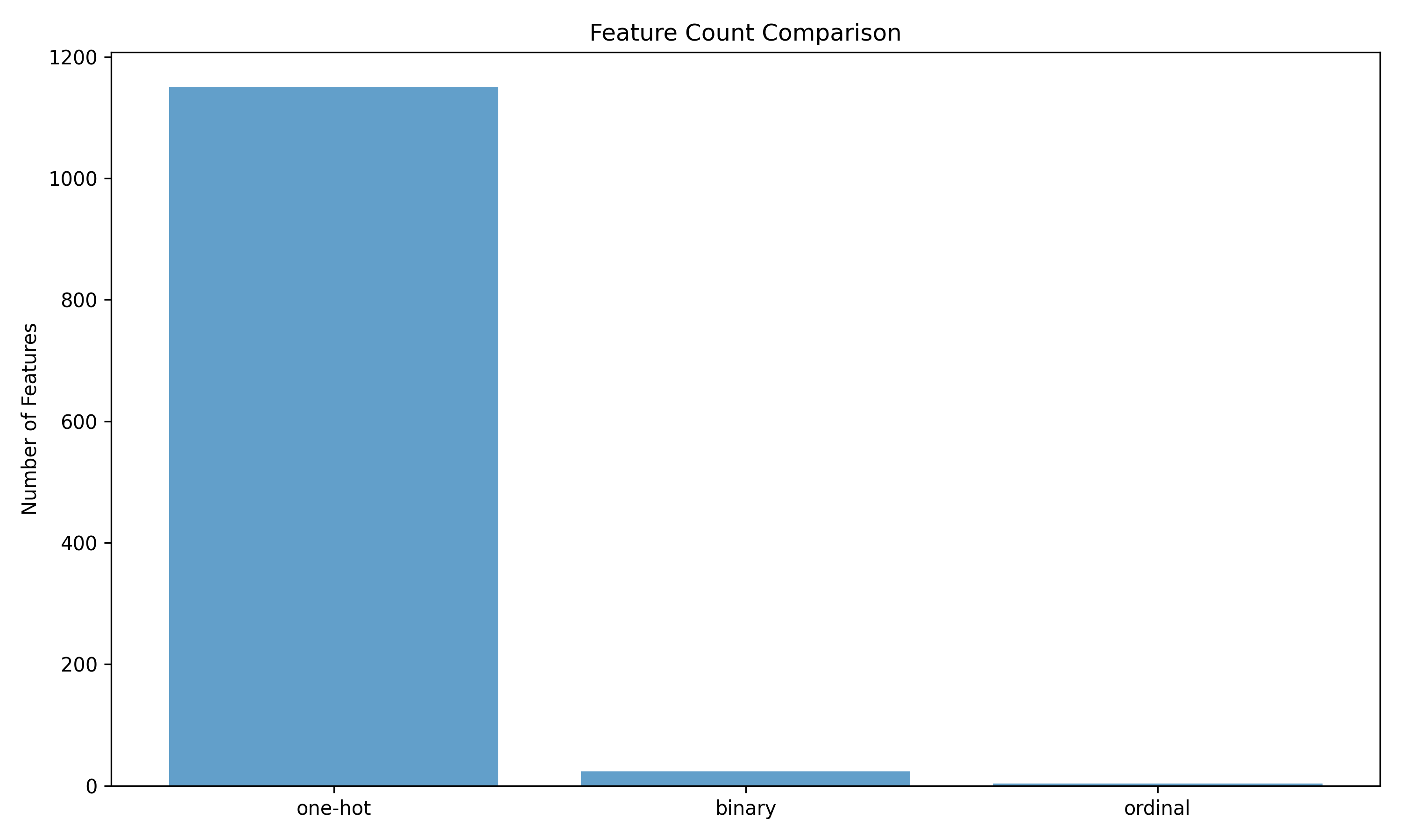
As you can see, binary encoding provides a good balance between feature count and model performance. One-hot encoding creates many more features, while ordinal encoding creates the fewest but may not capture the relationships as well.
When Binary Encoding Shines
Binary encoding is particularly effective in certain scenarios:
Extremely High-cardinality features: When dealing with categorical variables that have many unique values
Memory constraints: When working with limited memory or when model training time is a concern
No natural ordering: When categories don’t have a natural order, but one-hot encoding would create too many features
Tree-based models: Decision trees, random forests, and gradient boosting machines can often work well with binary encoding
New Category handling: By over-allocating space, it’s easy to accomodate new categories over time
Limitations and Considerations
While powerful, binary encoding has some limitations to be aware of:
Loss of interpretability: The binary columns don’t have a clear interpretation like one-hot encoded columns
Potential information loss: Some algorithms might not easily recover the original categorical information from the binary representation
Correlation introduction: The binary columns are not independent like one-hot encoded columns, which might affect some algorithms
Arbitrary mapping: Like ordinal encoding, the initial mapping from categories to integers is arbitrary unless specified
Problems with feature selection: Because of the way the features are created, treating them as independent for things like feature selection is at best problematic.
When to Use (and When Not to Use) Binary Encoding
Use binary encoding when:
- You have so many categories, which can update and expand over time, that you literlaly cannot use other methods
Consider alternatives when:
- Interpretability is crucial
- You’re working with linear models (one-hot might be better)
- Your categorical variables have few unique values
- Your categories have a natural ordering (ordinal might be better)
- You can use more advanced methods
Conclusion: The Compromise
Binary encoding offers an elegant compromise between the extreme approaches of one-hot and ordinal encoding. By representing categories as binary code, it achieves a much more compact representation than one-hot encoding while avoiding some of the drawbacks of ordinal encoding.
For high-cardinality features, the space savings can be substantial - potentially reducing hundreds or thousands of columns to just a handful. This efficiency makes binary encoding a valuable tool in your feature engineering toolkit, especially when working with large datasets or complex models.
In our next post, we’ll explore HashingEncoder, another space-efficient approach that uses hashing tricks to handle categorical variables.
Stay in the loop
Get notified when I publish new posts. No spam, unsubscribe anytime.