HashingEncoder: Tackling Extreme Cardinality with the Hashing Trick
In our journey through categorical encoding techniques, we’ve explored OneHotEncoder, OrdinalEncoder, and BinaryEncoder. Today, we’ll tackle an approach designed for extreme cardinality: the HashingEncoder from category_encoders.
When you’re dealing with millions of unique categories or streaming data where new categories appear constantly, traditional encoding methods break down. That’s where the hashing trick comes in.
The Challenge: Extreme Cardinality and Unknown Categories
Imagine you’re building a recommendation system for a platform with millions of products, or processing natural language data with an essentially unlimited vocabulary. In these scenarios, even binary encoding becomes unwieldy, and maintaining a mapping for every possible category is impractical or impossible.
The hashing trick offers a clever solution to this problem by:
- Using a fixed number of output features regardless of the number of categories
- Handling new, previously unseen categories automatically
- Requiring no storage of the mapping between categories and encoded features
How the Hashing Trick Works
The hashing encoder follows these steps:
- Apply a hash function to each category value
- Take the modulo of the hash with the desired number of output dimensions
- Create a binary or count-based feature vector based on these hash values
For example, with 3 output dimensions:
| Category | Hash Value | Hash % 3 | Encoded Vector |
|---|---|---|---|
| “apple” | 7213728 | 1 | [0, 1, 0] |
| “banana” | 9573927 | 0 | [1, 0, 0] |
| “cherry” | 2387498 | 2 | [0, 0, 1] |
| “date” | 8729742 | 1 | [0, 1, 0] |
Notice that “apple” and “date” hash to the same output dimension, causing a collision. This is a fundamental trade-off in hashing: we gain efficiency and flexibility at the cost of some information loss through collisions.
Implementation with category_encoders
The category_encoders library provides a powerful implementation of hashing encoding:
import pandas as pd
import category_encoders as ce
import numpy as np
import matplotlib.pyplot as plt
import seaborn as sns

# Sample data
data = pd.DataFrame({
    'color': ['red', 'blue', 'green', 'yellow', 'orange', 'purple', 'red', 'green'],
    'size': ['small', 'medium', 'large', 'medium', 'small', 'large', 'medium', 'small'],
    'price': [10.5, 15.0, 20.0, 18.5, 12.0, 22.5, 11.0, 19.5]
})

# Initialize the encoder with n_components=4
encoder = ce.HashingEncoder(cols=['color', 'size'], n_components=4)

# Fit and transform
encoded_data = encoder.fit_transform(data)
print(encoded_data)
This produces the following output:
   col_0  col_1  col_2  col_3  price
0      1      0      0      1   10.5
1      0      0      0      2   15.0
2      2      0      0      0   20.0
3      0      1      0      1   18.5
4      0      1      0      1   12.0
5      1      0      0      1   22.5
6      1      0      0      1   11.0
7      1      0      0      1   19.5
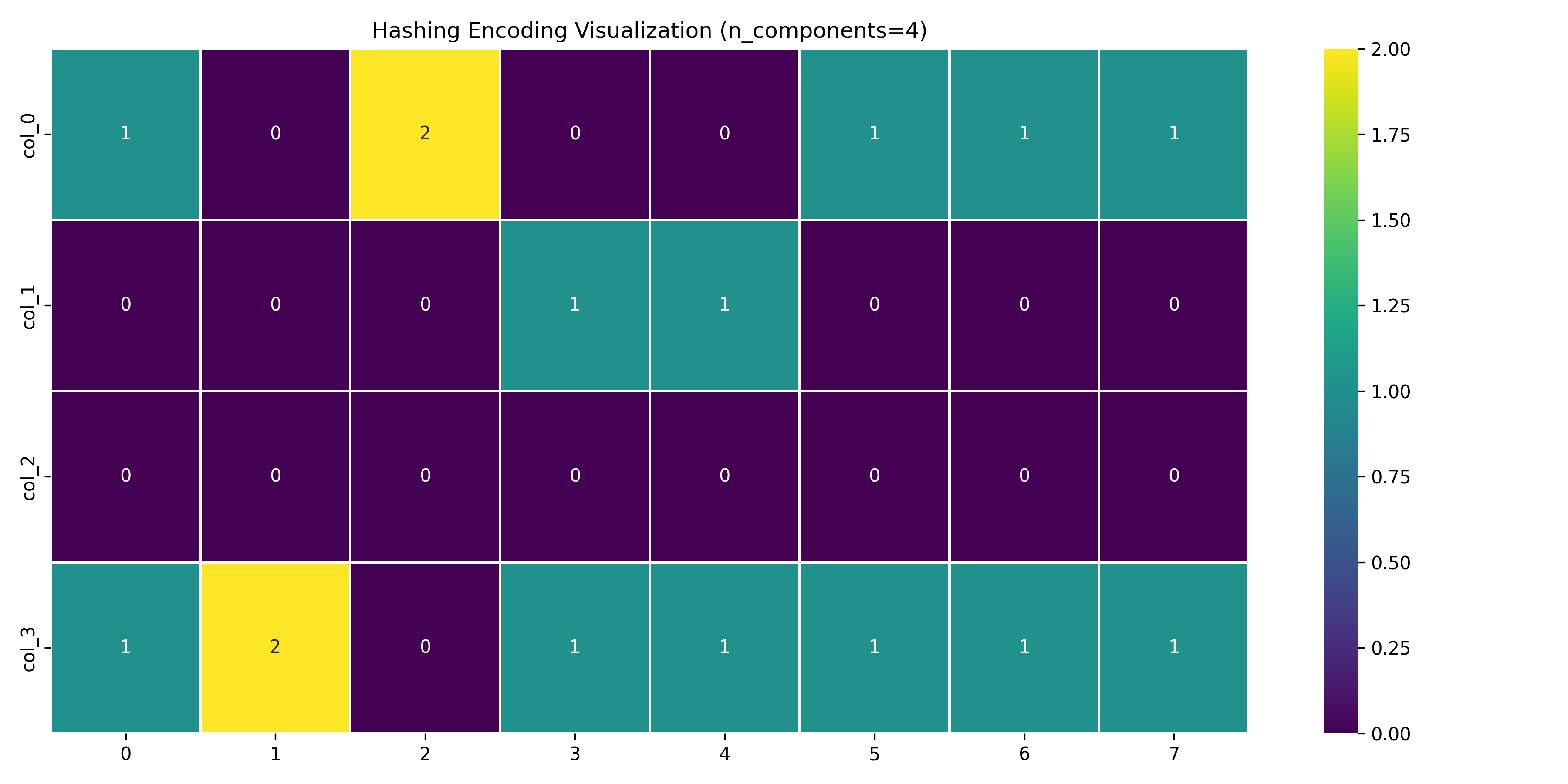
We can visualize this encoding with a heatmap:
# Visualize the encoding
plt.figure(figsize=(12, 6))
encoded_cols = [col for col in encoded_data.columns if col != 'price']
sns.heatmap(encoded_data[encoded_cols].T, cmap='viridis',
            annot=True, fmt='g', cbar=True, linewidths=1)
plt.title('Hashing Encoding Visualization (n_components=4)')
plt.tight_layout()
Collision Demonstration
One of the key aspects of hashing encoding is the trade-off between dimensionality and collision rate. Let’s demonstrate this with a larger dataset:
# Collision demonstration
np.random.seed(42)
n_samples = 100
colors = [f'color_{i}' for i in range(20)]  # 20 unique colors
sizes = [f'size_{i}' for i in range(10)]    # 10 unique sizes

large_data = pd.DataFrame({
    'color': np.random.choice(colors, n_samples),
    'size': np.random.choice(sizes, n_samples),
    'value': np.random.normal(0, 1, n_samples)
})

# Encode with different n_components
n_components_list = [2, 4, 8, 16]
for n in n_components_list:
    encoder = ce.HashingEncoder(cols=['color', 'size'], n_components=n)
    encoded = encoder.fit_transform(large_data)
    print(f"n_components={n}, shape={encoded.shape}")
Output:
n_components=2, shape=(100, 3)
n_components=4, shape=(100, 5)
n_components=8, shape=(100, 9)
n_components=16, shape=(100, 17)
As you can see, the number of output columns is directly related to the n_components parameter, which controls the dimensionality of the encoded space.
Key Features of category_encoders.HashingEncoder
The HashingEncoder in category_encoders offers several important parameters:
1. n_components
This controls the dimensionality of the output space:
# Create a more compact representation with 4 components
encoder = ce.HashingEncoder(cols=['product', 'color'], n_components=4)
2. hash_method
You can specify different hash functions:
# Use the md5 hash function
encoder = ce.HashingEncoder(cols=['product', 'color'], hash_method='md5')
3. Working with pandas DataFrames
# Direct support for pandas DataFrames
encoded_df = encoder.fit_transform(df)
The Math: Collisions and the Birthday Paradox
Hash collisions occur when different categories map to the same output feature. The probability of collisions is related to the birthday paradox and can be approximated as:
P(collision) ≈ 1 - e^(-k²/2n)
Where:
- k is the number of unique categories
- n is the number of output dimensions
For example, with 100 unique categories and 1,000 output dimensions, the probability of at least one collision is about 0.993 or 99.3%.
This means collisions are practically inevitable with large numbers of categories, but their impact can be minimized by:
- Using a sufficient number of output dimensions
- Employing a good hash function that distributes values uniformly
- Leveraging the fact that most machine learning algorithms can handle some noise in the features
Real-World Example: Text Classification with High-Dimensional Features
Let’s use HashingEncoder in a practical scenario - classifying text documents with a large vocabulary:
import pandas as pd
import category_encoders as ce
import numpy as np
from sklearn.model_selection import train_test_split
from sklearn.ensemble import RandomForestClassifier
from sklearn.metrics import classification_report
from sklearn.feature_extraction.text import CountVectorizer

# Sample text data (simplified for illustration)
np.random.seed(42)
n_samples = 1000

# Generate synthetic data - imagine these are product reviews
categories = ['electronics', 'clothing', 'books', 'home', 'sports']
sentiments = ['positive', 'negative', 'neutral']

# Create a dataset with text and categorical features
data = pd.DataFrame({
    'text': [f"This is sample text {i}" for i in range(n_samples)],
    'category': np.random.choice(categories, n_samples),
    'user_id': [f"user_{np.random.randint(1, 10000)}" for _ in range(n_samples)],
    'sentiment': np.random.choice(sentiments, n_samples)
})

# Extract word counts from text
vectorizer = CountVectorizer(max_features=1000)
text_features = vectorizer.fit_transform(data['text'])
text_df = pd.DataFrame(text_features.toarray(),
                       columns=[f'word_{i}' for i in range(text_features.shape[1])])

# Use HashingEncoder for high-cardinality user_id
encoder = ce.HashingEncoder(cols=['user_id'], n_components=50)
user_encoded = encoder.fit_transform(data[['user_id']])

# Use OneHotEncoder for low-cardinality category
cat_encoder = ce.OneHotEncoder(cols=['category'])
category_encoded = cat_encoder.fit_transform(data[['category']])

# Combine all features
X = pd.concat([text_df.reset_index(drop=True),
               user_encoded.reset_index(drop=True),
               category_encoded.reset_index(drop=True)], axis=1)
y = data['sentiment']

# Split the data
X_train, X_test, y_train, y_test = train_test_split(X, y, test_size=0.2, random_state=42)

# Train a model
model = RandomForestClassifier(n_estimators=100, random_state=42)
model.fit(X_train, y_train)

# Make predictions
y_pred = model.predict(X_test)

# Evaluate
print(classification_report(y_test, y_pred))

# Feature importance analysis
feature_importance = pd.DataFrame({
    'feature': X.columns,
    'importance': model.feature_importances_
}).sort_values('importance', ascending=False).head(20)

print("\nTop 20 Features by Importance:")
print(feature_importance)
This example demonstrates how HashingEncoder can be used to handle high-cardinality features (like user IDs) in a text classification task, combining it with other encoding techniques for different feature types.
When HashingEncoder Shines
HashingEncoder is particularly effective in certain scenarios:
Extreme cardinality: When dealing with categorical variables that have thousands or millions of unique values
Online learning: When processing streaming data where new categories appear over time
Memory constraints: When you can’t afford to store a mapping for every category
Privacy concerns: When you want to avoid storing the original categorical values
Limitations and Considerations
While powerful, the hashing trick has some important limitations:
Collisions: Different categories can map to the same feature, potentially reducing model performance
Irreversibility: You can’t easily convert back from the hashed representation to the original categories
Feature interpretation: The hashed features don’t have a clear interpretation, making the model less explainable
Tuning required: The number of components needs to be tuned to balance dimensionality and collision rate
When to Use (and When Not to Use) HashingEncoder
Use HashingEncoder when:
- You have extremely high-cardinality features
- You’re working with streaming data where new categories appear over time
- Memory efficiency is critical
- You don’t need to interpret individual features
- You can tolerate some information loss
Consider alternatives when:
- Your categorical variables have relatively few unique values
- Interpretability is crucial
- You need to convert back to the original categories
- You can’t afford any information loss from collisions
Conclusion: The Scalable Solution for Extreme Cardinality
HashingEncoder represents a clever solution to the challenge of extreme cardinality in categorical features. By using the hashing trick, it provides a fixed-size representation regardless of the number of unique categories, handles new categories automatically, and requires minimal memory.
While it introduces some information loss through collisions, this trade-off is often acceptable given the substantial benefits in scalability and flexibility. For applications with millions of unique categories or streaming data, HashingEncoder may be not just the best option but the only practical one.
In our next post, we’ll explore TargetEncoder, which takes a completely different approach by incorporating the target variable into the encoding process.
Stay in the loop
Get notified when I publish new posts. No spam, unsubscribe anytime.