The Glicko Rating System: When Confidence Matters

Exploring Ideas: A Blog on Technology, Startups, Food, and More

In our previous post, we explored the Elo rating system - the grandfather of competitive rankings. While Elo is elegant in its simplicity, it has some limitations. One of the biggest is that it treats all ratings as equally reliable, whether they’re based on thousands of games or just a handful.

Enter the Glicko rating system, which addresses this limitation by tracking not just a player’s rating, but also how confident we should be in that rating.

The Origin Story: Improving on Elo

The Glicko rating system was developed by Mark Glickman (hence the name) in the late 1990s. As a statistician and chess player, Glickman recognized that Elo’s one-dimensional approach to ratings was missing something important: uncertainty.

Consider two chess players with the same 1500 Elo rating:

Player A has played 1,000 games, with their rating stable around 1500 for years
Player B is new and has only played 10 games

Should we have the same confidence in both ratings? Intuitively, no - and Glickman formalized this intuition into the Glicko system.

How Glicko Works: Adding the Uncertainty Dimension

Glicko builds on Elo by adding a second parameter: Rating Deviation (RD). This parameter represents the uncertainty in a player’s rating:

Every player has both a rating (like in Elo) and a rating deviation
New players start with a high RD, indicating high uncertainty
As players compete, their RD decreases (more certainty)
During periods of inactivity, RD gradually increases (less certainty)
When calculating expected outcomes, RD is factored in

Let’s see how this works in practice with Elote:

Basic Example: A Single Match

Here’s a simple example showing how ratings and RDs change after a match:

from elote import GlickoCompetitor
import datetime

# Create two competitors
player_a = GlickoCompetitor()  # Default rating=1500, rd=350
player_b = GlickoCompetitor()

# Check initial ratings
print(f"Initial ratings - Player A: {player_a.rating}, RD: {player_a.rd}")
print(f"Initial ratings - Player B: {player_b.rating}, RD: {player_b.rd}")

# Record a match result with a timestamp
match_timestamp = datetime.datetime.now()
player_a.beat(player_b, match_time=match_timestamp)

# See how ratings and RDs changed
print(f"After Player A beats Player B - Player A: {player_a.rating}, RD: {player_a.rd}")
print(f"After Player A beats Player B - Player B: {player_b.rating}, RD: {player_b.rd}")

Which prints:

Initial ratings - Player A: 1500, RD: 350
Initial ratings - Player B: 1500, RD: 350
After Player A beats Player B - Player A: 1500.9068905933125, RD: 349.99882506078484
After Player A beats Player B - Player B: 1499.0931094066875, RD: 349.99882506078484

Notice how both the ratings and RDs change after the match. The winner’s rating increases, the loser’s decreases, and both players’ RDs decrease (we’re more certain about their skill levels).

Rating Deviation Decay

One of Glicko’s key features is how it handles player inactivity. The longer a player goes without competing, the less certain we become about their true skill level. Elote v1.1.0 and later uses actual timestamps provided with each match result (match_time) to calculate this decay more accurately based on the real time elapsed, rather than just counting periods of inactivity.

import matplotlib.pyplot as plt
import numpy as np
import datetime

def simulate_rd_decay(initial_rd, periods, c=34.64):
    """Simulate RD decay over periods of inactivity"""
    rd = initial_rd
    rd_history = [rd]
    
    for _ in range(periods):
        rd = min(350, np.sqrt(rd**2 + c**2))
        rd_history.append(rd)
    
    return rd_history

# Plot RD decay for different initial RDs
periods = 20
initial_rds = [50, 100, 200, 350]
plt.figure(figsize=(10, 6))

for initial_rd in initial_rds:
    rd_history = simulate_rd_decay(initial_rd, periods)
    plt.plot(range(periods+1), rd_history, marker='o', label=f'Initial RD={initial_rd}')

plt.axhline(y=350, color='r', linestyle='--', alpha=0.5, label='Maximum RD (350)')
plt.xlabel('Periods of Inactivity')
plt.ylabel('Rating Deviation (RD)')
plt.title('Glicko Rating Deviation Decay Over Time')
plt.legend()
plt.grid(True, alpha=0.3)

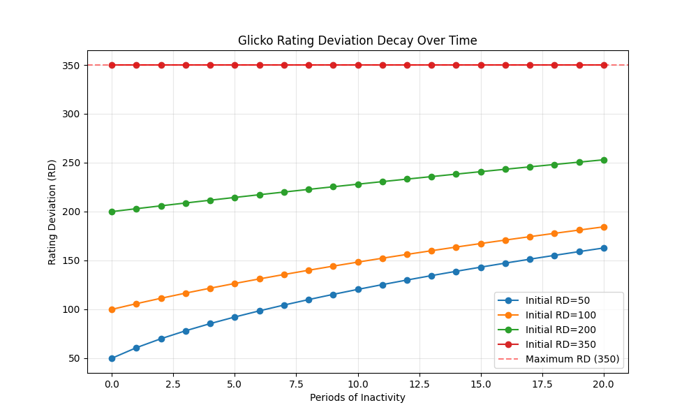
This chart shows how rating deviation increases during periods of inactivity. The longer a player goes without competing, the less certain we are about their true skill level, up to a maximum RD of 350.

Win Probability with Different RDs

The RD values affect how we calculate win probabilities. When we’re uncertain about players’ ratings (high RD), our win probability predictions become more conservative (closer to 50/50). Let’s compare a scenario where both players have high certainty (low RD = 50) with one where both have low certainty (high RD = 350):

# Visualize win probability with different RDs
rating_diffs = np.arange(-400, 401, 20)
# Compare low RD vs high RD directly
rd_values = [
    50,    # Low RD (high certainty)
    350   # High RD (low certainty)
]

plt.figure(figsize=(10, 6))

for rd in rd_values:
    win_probs = []
    for diff in rating_diffs:
        # Assume both players have the same RD for simplicity
        player = GlickoCompetitor(initial_rating=1500, initial_rd=rd)
        opponent = GlickoCompetitor(initial_rating=1500 + diff, initial_rd=rd)
        win_probs.append(player.expected_score(opponent))
    
    plt.plot(rating_diffs, win_probs, 
             label=f'Both Players RD={rd}')

plt.axhline(y=0.5, color='r', linestyle='--', alpha=0.5)
plt.axvline(x=0, color='r', linestyle='--', alpha=0.5)
plt.grid(True, alpha=0.3)
plt.xlabel('Rating Difference (Player - Opponent)')
plt.ylabel('Win Probability')
plt.title('Glicko Win Probability vs. Rating Difference for Different RDs')
plt.legend()

This visualization demonstrates how RD affects win probability calculations. When both players have high uncertainty (high RD), the win probability curve flattens, reflecting our reduced confidence in the outcome prediction compared to the high certainty (low RD) case.

Comparing Glicko with Elo

Let’s see how Glicko’s win probabilities differ from Elo’s. We’ll compare standard Elo with Glicko using a very low RD (approximating high certainty) and a high RD (representing low certainty):

from elote import EloCompetitor

rating_diffs = np.arange(-400, 401, 20)
win_probs_elo = []
win_probs_glicko_certain = []
win_probs_glicko_uncertain = []

for diff in rating_diffs:
    # Elo
    elo_player = EloCompetitor(initial_rating=1500)
    elo_opponent = EloCompetitor(initial_rating=1500 + diff)
    win_probs_elo.append(elo_player.expected_score(elo_opponent))
    
    # Glicko with very low RD (very high certainty, approximates Elo)
    glicko_certain_player = GlickoCompetitor(initial_rating=1500, initial_rd=25) # Use RD=25 for high certainty
    glicko_certain_opponent = GlickoCompetitor(initial_rating=1500 + diff, initial_rd=25) # Use RD=25 for high certainty
    win_probs_glicko_certain.append(glicko_certain_player.expected_score(glicko_certain_opponent))
    
    # Glicko with high RD (low certainty)
    glicko_uncertain_player = GlickoCompetitor(initial_rating=1500, initial_rd=350)
    glicko_uncertain_opponent = GlickoCompetitor(initial_rating=1500 + diff, initial_rd=350)
    win_probs_glicko_uncertain.append(glicko_uncertain_player.expected_score(glicko_uncertain_opponent))

plt.figure(figsize=(10, 6))
plt.plot(rating_diffs, win_probs_elo, label='Elo')
plt.plot(rating_diffs, win_probs_glicko_certain, label='Glicko (Low RD)')
plt.plot(rating_diffs, win_probs_glicko_uncertain, label='Glicko (High RD)')

plt.axhline(y=0.5, color='r', linestyle='--', alpha=0.5)
plt.axvline(x=0, color='r', linestyle='--', alpha=0.5)
plt.grid(True, alpha=0.3)
plt.xlabel('Rating Difference (Player - Opponent)')
plt.ylabel('Win Probability')
plt.title('Elo vs. Glicko Win Probability')
plt.legend()

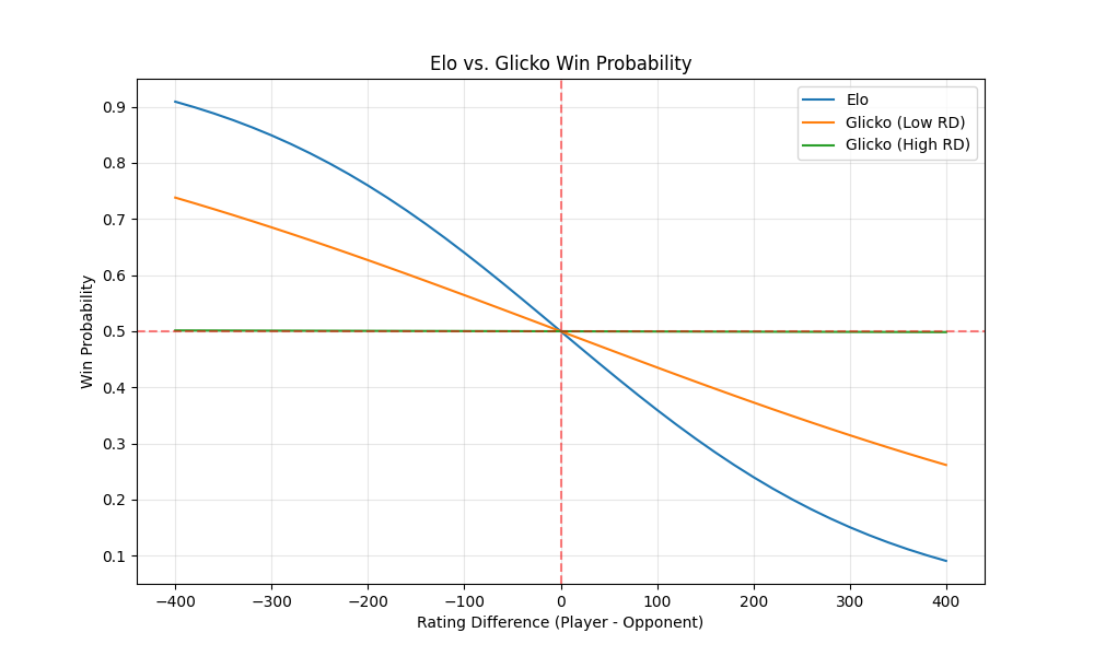
This comparison shows how Glicko’s win probabilities differ from Elo’s. With very high certainty (very low RD, here RD=25), Glicko behaves very similarly to Elo, showing a steep curve based on rating difference. With low certainty (high RD), Glicko produces a much flatter curve, indicating less confidence in the outcome.

Rating Changes After Matches

Let’s examine how ratings change after wins against opponents of different strengths:

import datetime

# Visualize rating changes
rating_diffs = np.arange(-400, 401, 20)
rd_values = [50, 150, 350]
rating_changes = {}

base_time = datetime.datetime.now()
for rd in rd_values:
    changes = []
    for i, diff in enumerate(rating_diffs):
        player = GlickoCompetitor(initial_rating=1500, initial_rd=rd)
        opponent = GlickoCompetitor(initial_rating=1500 + diff, initial_rd=rd)
        initial_rating = player.rating
        match_timestamp = base_time + datetime.timedelta(days=i)
        player.beat(opponent, match_time=match_timestamp)
        changes.append(player.rating - initial_rating)
    rating_changes[rd] = changes

plt.figure(figsize=(10, 6))
for rd, changes in rating_changes.items():
    plt.plot(rating_diffs, changes, label=f'RD={rd}')

plt.axhline(y=0, color='r', linestyle='--', alpha=0.5)
plt.axvline(x=0, color='r', linestyle='--', alpha=0.5)
plt.grid(True, alpha=0.3)
plt.xlabel('Rating Difference (Opponent - Player)')
plt.ylabel('Rating Change After Win')
plt.title('Glicko Rating Change vs. Rating Difference for Different RDs')
plt.legend()

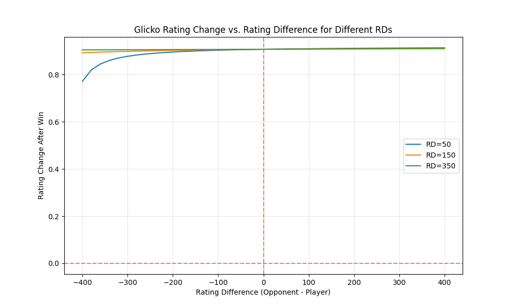
This chart shows how a player’s rating changes after winning against opponents of different strengths. Notice how the RD affects the magnitude of rating changes - higher RD leads to larger rating shifts.

RD Changes After Matches

Finally, let’s look at how RD changes after matches:

import datetime

# Visualize RD changes after matches
rd_changes = {}
base_time = datetime.datetime.now()
for rd in rd_values:
    changes = []
    for i, diff in enumerate(rating_diffs):
        player = GlickoCompetitor(initial_rating=1500, initial_rd=rd)
        opponent = GlickoCompetitor(initial_rating=1500 + diff, initial_rd=rd)
        initial_rd = player.rd
        match_timestamp = base_time + datetime.timedelta(days=i)
        player.beat(opponent, match_time=match_timestamp)
        changes.append(player.rd - initial_rd)
    rd_changes[rd] = changes

plt.figure(figsize=(10, 6))
for rd, changes in rd_changes.items():
    plt.plot(rating_diffs, changes, label=f'Initial RD={rd}')

plt.axhline(y=0, color='r', linestyle='--', alpha=0.5)
plt.axvline(x=0, color='r', linestyle='--', alpha=0.5)
plt.grid(True, alpha=0.3)
plt.xlabel('Rating Difference (Opponent - Player)')
plt.ylabel('RD Change After Match')
plt.title('Glicko RD Change vs. Rating Difference')
plt.legend()

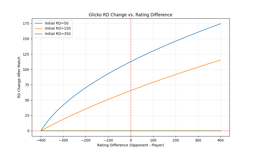
This visualization shows how RD decreases after matches, with the amount of decrease varying based on the initial RD and the rating difference between players.

Pros and Cons of the Glicko-1 System

Pros:

Tracks uncertainty: Distinguishes between reliable and unreliable ratings
Handles inactivity: Ratings become more uncertain over time without matches
More accurate for new players: Ratings stabilize faster than with Elo
Still relatively simple: Only slightly more complex than Elo
Provides confidence intervals: Can show rating ranges, not just point estimates

Cons:

More complex: Requires tracking and updating an additional parameter
Still has limitations for teams: Like Elo, doesn’t model team dynamics well
Update frequency matters: Works best when ratings are updated after each match
Doesn’t track volatility: Some players’ performances are more consistent than others

When to Use Glicko-1

Glicko-1 is best when:

You need more accurate ratings than Elo provides
Players compete with varying frequency
You want to express confidence in ratings
The pool of competitors changes over time (new players join, others become inactive)
You’re willing to accept a bit more complexity than Elo

Conclusion: The Value of Knowing What You Don’t Know

The key insight of Glicko-1 is that knowing the limits of your knowledge is valuable. By tracking not just skill estimates but also their reliability, Glicko-1 provides a more nuanced and accurate rating system than Elo.

In our next post, we’ll explore Glicko-2, which builds on Glicko-1 by adding a third parameter to track player volatility - how consistently a player performs.

Until then, may your ratings be high and your deviations low!

Subscribe to the Newsletter

Get the latest posts and insights delivered straight to your inbox.