Bankroll Management with Keeks: OptimalF
In our previous posts, we explored the Kelly Criterion, Fractional Kelly, and Drawdown-Adjusted Kelly strategies. Today, we’ll examine OptimalF, a different approach to bankroll management developed by trading system expert Ralph Vince.
What is OptimalF?
OptimalF is a position sizing method developed by Ralph Vince in the late 1980s as an alternative to the Kelly Criterion. While Kelly focuses on maximizing the expected logarithm of wealth, OptimalF aims to maximize the geometric growth rate of your bankroll based on your historical trading or betting results.
The key difference is that OptimalF doesn’t require you to know the probability of winning in advance. Instead, it works backward from your actual trading history to determine the optimal fraction of your bankroll to risk on each bet.
The Theory Behind OptimalF
OptimalF is based on the concept of the Terminal Wealth Relative (TWR), which is the final value of your bankroll divided by its initial value after a series of bets. The geometric mean of these wealth relatives over many bets is what OptimalF seeks to maximize.
For a series of trades or bets, the formula for TWR is:
TWR = (1 + f*R₁) * (1 + f*R₂) * ... * (1 + f*Rₙ)
Where:
fis the fraction of your bankroll risked on each betRᵢis the return on the i-th bet as a fraction of the amount risked
OptimalF finds the value of f that maximizes this product, typically through numerical methods rather than a closed-form solution.
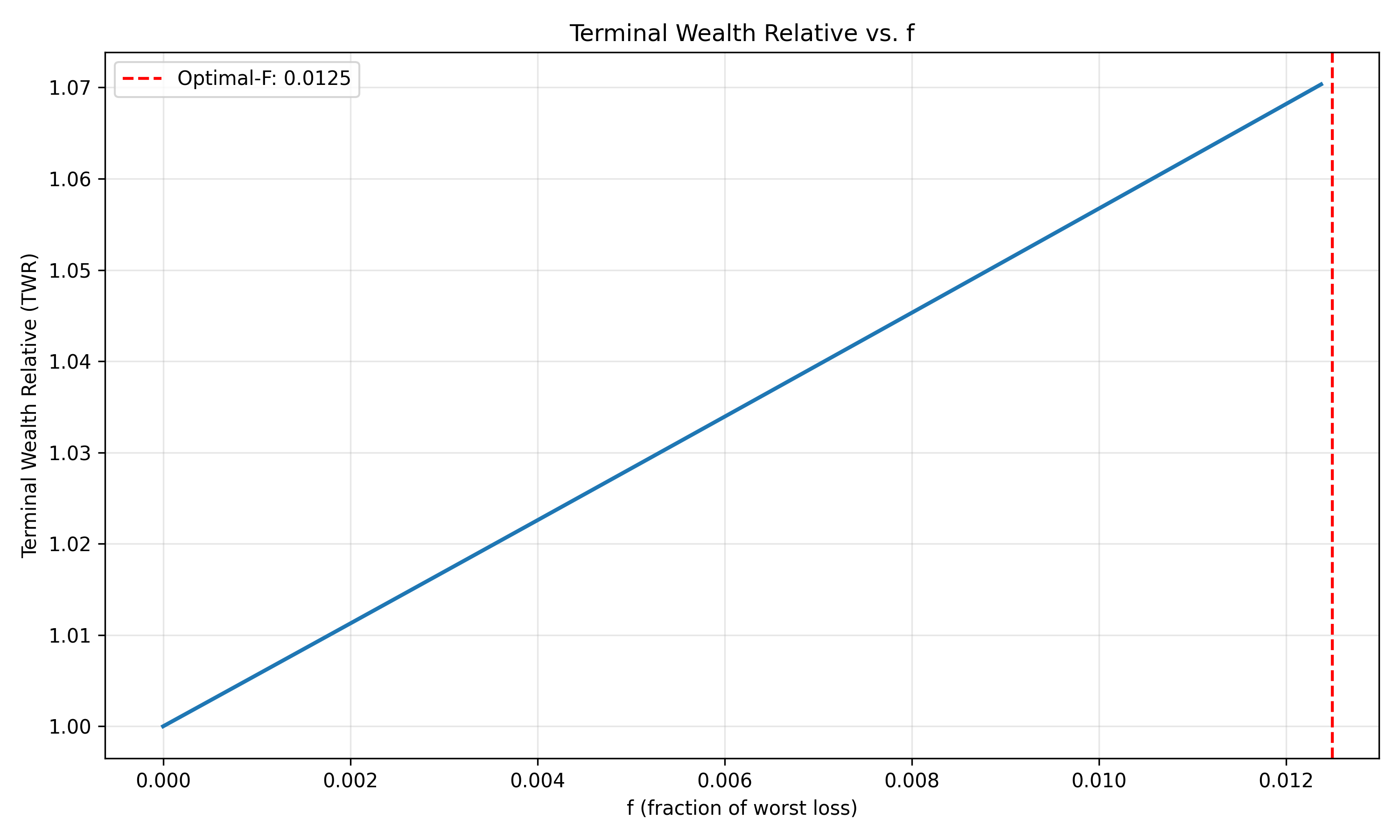
The graph above shows how the Terminal Wealth Relative (TWR) changes with different values of f. The peak of this curve represents the OptimalF value.
Pros of OptimalF
- Works with historical data: Doesn’t require accurate probability estimates
- Adapts to your specific trading/betting style: Customized to your actual results
- Accounts for varying payoffs: Handles bets with different risk/reward ratios
- Robust to outliers: Less sensitive to extreme wins or losses than simple averages
- Practical for complex scenarios: Works well for systems with multiple bet types
Cons of OptimalF
- Backward-looking: Assumes future performance will resemble past performance
- Computationally intensive: Requires numerical optimization rather than a simple formula
- Sample size sensitivity: Needs sufficient historical data to be reliable
- Can be aggressive: Often recommends larger position sizes than Kelly
Implementing OptimalF with Keeks
The keeks library provides an OptimalF strategy that handles the TWR optimization for you. Let’s see how it works:
from keeks.bankroll import BankRoll
from keeks.binary_strategies.optimalf import OptimalF
from keeks.simulators.repeated_binary import RepeatedBinarySimulator

# Simulation parameters
PAYOFF = 1.0
LOSS = 1.0
PROBABILITY = 0.55
TRIALS = 1000

# Create an OptimalF strategy
strategy = OptimalF(payoff=PAYOFF, loss=LOSS, transaction_cost=0)

# Set up bankroll and simulator
bankroll = BankRoll(initial_funds=10000.0, max_draw_down=0.5)
simulator = RepeatedBinarySimulator(
    payoff=PAYOFF,
    loss=LOSS,
    transaction_costs=0,
    probability=PROBABILITY,
    trials=TRIALS
)

# Run the simulation
simulator.evaluate_strategy(strategy, bankroll)

print(f"Initial bankroll: $10,000.00")
print(f"Final bankroll: ${bankroll.total_funds:.2f}")
print(f"Peak bankroll: ${max(bankroll.history):.2f}")
The OptimalF strategy in keeks handles the geometric growth optimization internally, making it easy to use alongside other strategies.
Comparing OptimalF with Kelly Criterion
Let’s compare OptimalF with the Kelly Criterion using keeks:
from keeks.bankroll import BankRoll
from keeks.binary_strategies.kelly import KellyCriterion
from keeks.binary_strategies.optimalf import OptimalF
from keeks.simulators.repeated_binary import RepeatedBinarySimulator

# Parameters
PAYOFF = 1.0
LOSS = 1.0
PROBABILITY = 0.6
TRIALS = 500

# Create strategies
kelly = KellyCriterion(payoff=PAYOFF, loss=LOSS, transaction_cost=0)
optimal_f = OptimalF(payoff=PAYOFF, loss=LOSS, transaction_cost=0)

# Create simulator
simulator = RepeatedBinarySimulator(
    payoff=PAYOFF,
    loss=LOSS,
    transaction_costs=0,
    probability=PROBABILITY,
    trials=TRIALS
)

# Compare both strategies
for name, strategy in [("Kelly", kelly), ("OptimalF", optimal_f)]:
    bankroll = BankRoll(initial_funds=1000.0, max_draw_down=0.5)
    simulator.evaluate_strategy(strategy, bankroll)
    print(f"{name}: Final bankroll ${bankroll.total_funds:.2f}")
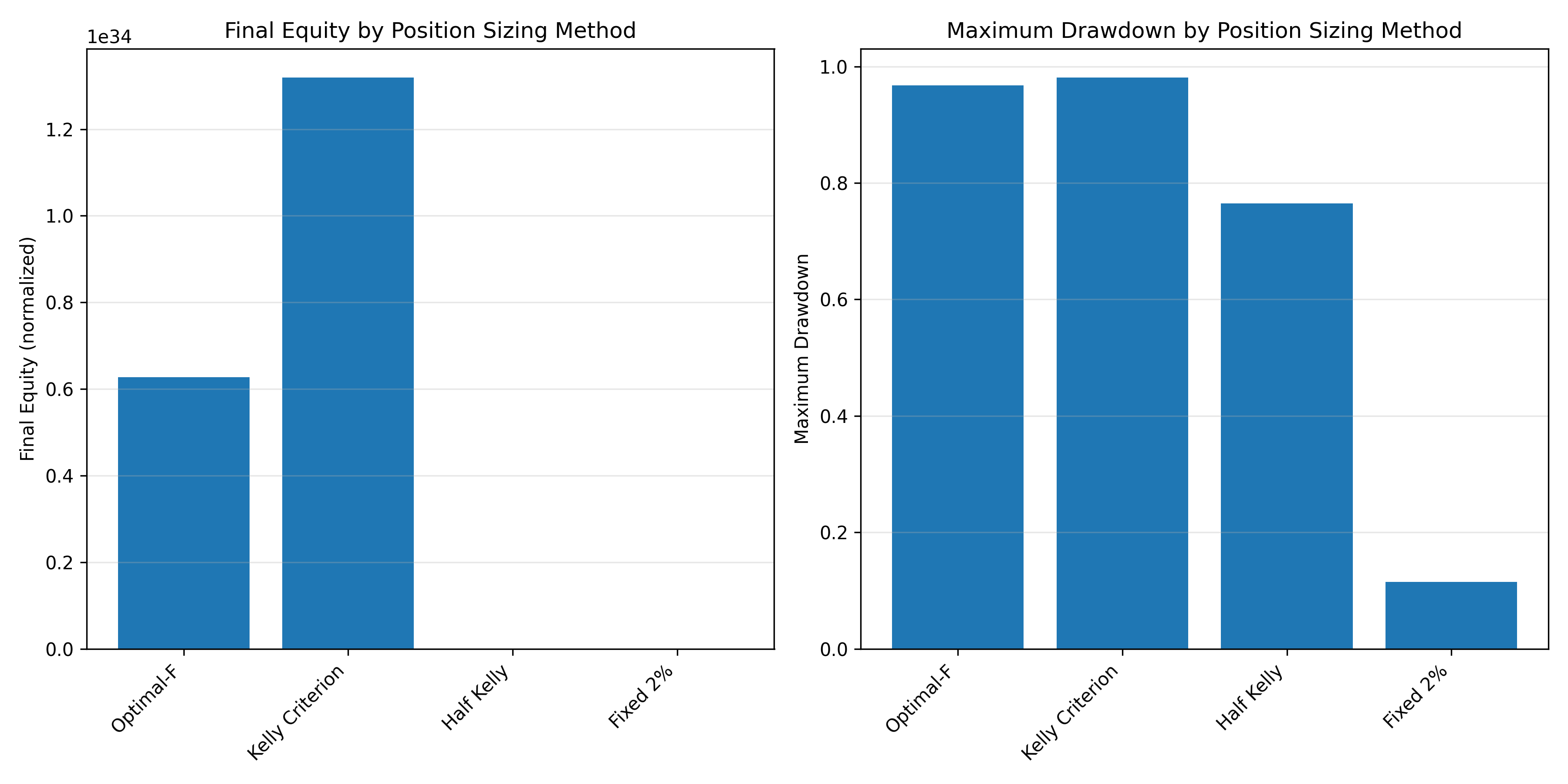
The chart above compares the performance of OptimalF with the Kelly Criterion and other position sizing methods. Notice that OptimalF often produces more aggressive position sizes, leading to higher potential returns but also greater volatility.
Simulating Trading with Different Position Sizing Methods
Let’s simulate trading with different position sizing methods using keeks:
from keeks.bankroll import BankRoll
from keeks.binary_strategies.kelly import KellyCriterion
from keeks.binary_strategies.fractional_kelly import FractionalKellyCriterion
from keeks.binary_strategies.optimalf import OptimalF
from keeks.binary_strategies.fixed_fraction import FixedFraction
from keeks.simulators.repeated_binary import RepeatedBinarySimulator

# Parameters
PAYOFF = 1.0
LOSS = 1.0
PROBABILITY = 0.6
TRIALS = 1000

# Create all strategies to compare
strategies = {
    "OptimalF": OptimalF(payoff=PAYOFF, loss=LOSS, transaction_cost=0),
    "Kelly": KellyCriterion(payoff=PAYOFF, loss=LOSS, transaction_cost=0),
    "Half Kelly": FractionalKellyCriterion(payoff=PAYOFF, loss=LOSS, transaction_cost=0, fraction=0.5),
    "Fixed 2%": FixedFraction(payoff=PAYOFF, loss=LOSS, transaction_cost=0, fraction=0.02),
}

# Create simulator
simulator = RepeatedBinarySimulator(
    payoff=PAYOFF,
    loss=LOSS,
    transaction_costs=0,
    probability=PROBABILITY,
    trials=TRIALS
)

# Run simulations
for name, strategy in strategies.items():
    bankroll = BankRoll(initial_funds=1000.0, max_draw_down=0.5)
    simulator.evaluate_strategy(strategy, bankroll)

    # Calculate max drawdown
    peak = bankroll.history[0]
    max_dd = 0
    for value in bankroll.history:
        if value > peak:
            peak = value
        elif peak > 0:
            dd = (peak - value) / peak
            max_dd = max(max_dd, dd)

    print(f"{name}:")
    print(f"  Final equity: ${bankroll.total_funds:.2f}")
    print(f"  Maximum drawdown: {max_dd:.2%}")
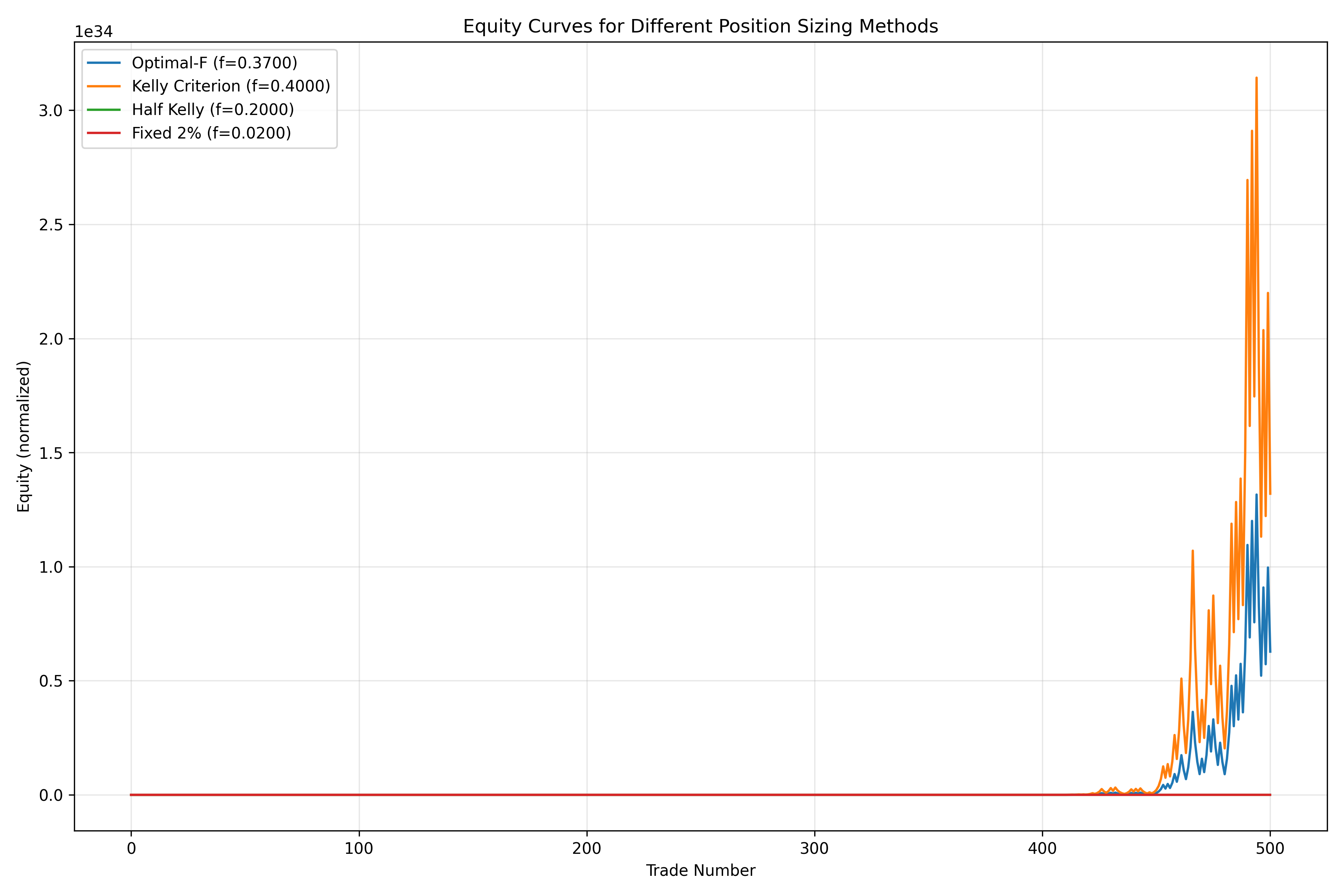
The equity curves show how each position sizing method performs over time. OptimalF often produces the highest final equity but with more significant drawdowns.
OptimalF with Different Trade Distributions
The performance of OptimalF can vary significantly depending on the distribution of your trades:
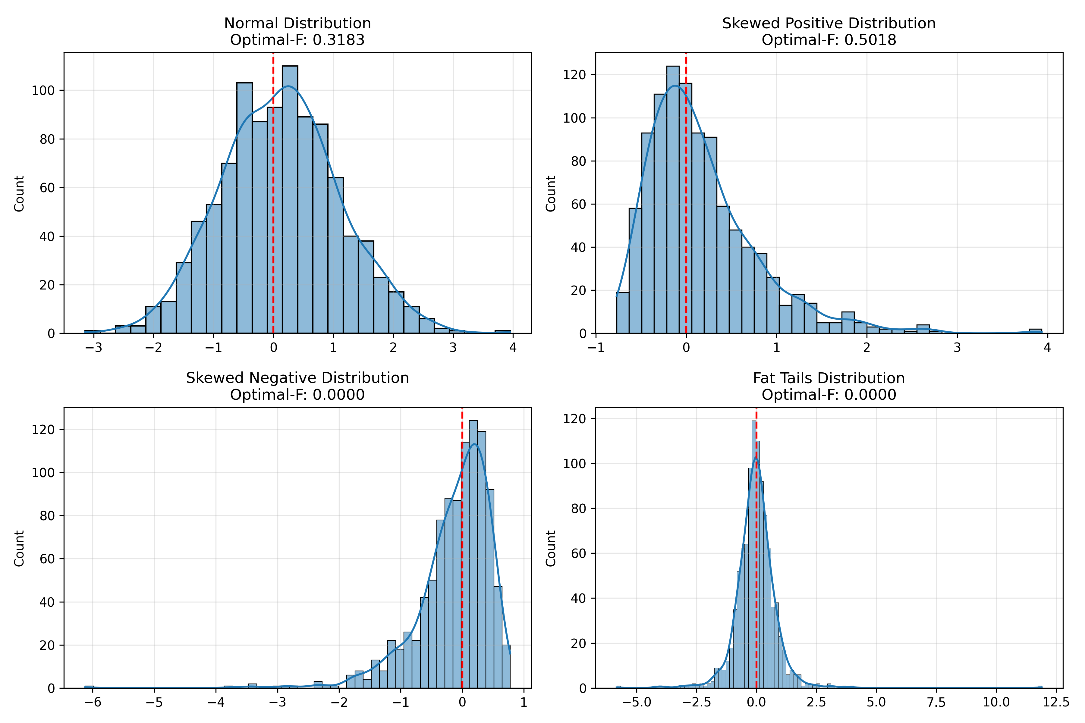
The chart above shows how OptimalF values change with different trade distributions. Notice that OptimalF is particularly sensitive to the presence of large losses in your trading history.
Practical Application: Position Sizing with OptimalF
Here’s a practical example of using OptimalF for position sizing using keeks:
from keeks.bankroll import BankRoll
from keeks.binary_strategies.optimalf import OptimalF

# Create an OptimalF strategy for trading
# Typical trade: 15% gain or 10% loss
strategy = OptimalF(payoff=0.15, loss=0.10, transaction_cost=0.001)

# Calculate position sizing for different account sizes
account_sizes = [10000, 50000, 100000]
win_probability = 0.55

for account_size in account_sizes:
    bankroll = BankRoll(initial_funds=float(account_size), max_draw_down=0.3)
    position_size = strategy.evaluate(win_probability, bankroll.total_funds)
    print(f"Account: ${account_size:,} -> Position size: ${position_size:,.2f}")
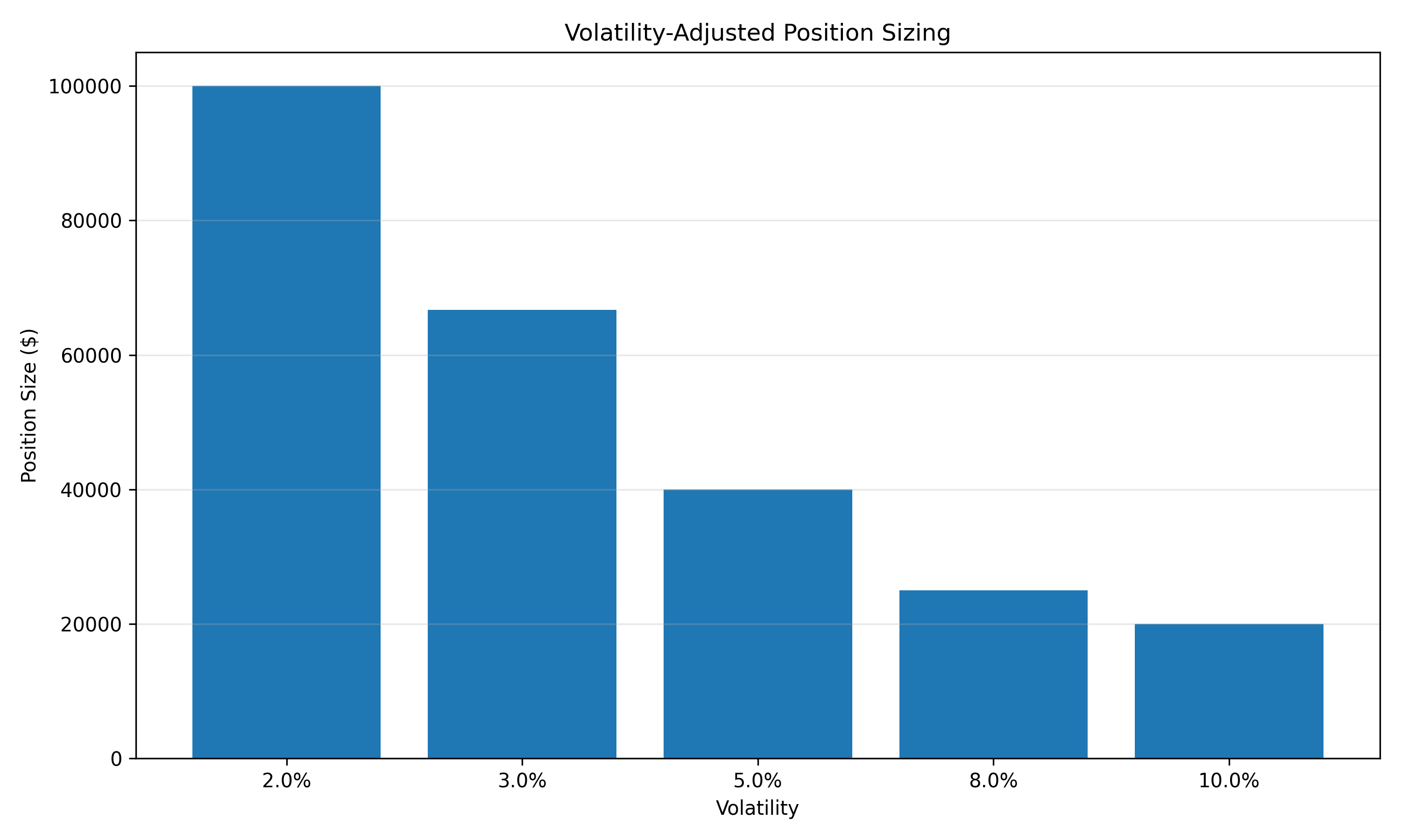
The chart above shows how position sizes should be adjusted based on market volatility. Higher volatility environments require smaller position sizes to maintain the same risk level.
When to Use OptimalF
OptimalF is particularly useful in the following scenarios:
When you have a significant trading history: OptimalF works best when you have a substantial number of historical trades to analyze.
For systems with varying payoffs: If your trading or betting system produces wins and losses of different magnitudes, OptimalF can handle this complexity better than simpler methods.
When probability estimates are unreliable: If you don’t have reliable estimates of win probabilities, OptimalF can work directly with your trading results.
For professional traders: OptimalF is popular among professional traders who need to maximize their growth rate while managing risk.
Practical Recommendations
Based on both theory and empirical evidence, here are some practical recommendations for using OptimalF:
Use a safety factor: Consider using 50-70% of the calculated OptimalF value to reduce volatility.
Regularly recalculate: Update your OptimalF value as you accumulate more trading history.
Be cautious with small samples: If you have fewer than 30-50 trades, OptimalF results may not be reliable.
Consider market conditions: Adjust your OptimalF value based on current market volatility and conditions.
Combine with drawdown control: Consider implementing drawdown limits alongside OptimalF to protect your capital during losing streaks.
Conclusion
OptimalF represents a powerful approach to position sizing that works directly with your trading history rather than requiring probability estimates. While it can be more aggressive than the Kelly Criterion, it offers a data-driven method for maximizing your long-term growth rate.
The key to using OptimalF successfully is understanding its limitations and implementing appropriate safety factors to manage risk. By combining OptimalF with proper risk management techniques, you can create a robust position sizing strategy tailored to your specific trading or betting style.
In our next post, we’ll explore Fixed Fraction position sizing, a simpler approach that offers consistency and predictability for risk management.
Stay in the loop
Get notified when I publish new posts. No spam, unsubscribe anytime.