Bankroll Management with Keeks: Fixed Fraction

In our previous posts, we’ve explored mathematically sophisticated bankroll management strategies like the Kelly Criterion, Fractional Kelly, Drawdown-Adjusted Kelly, and OptimalF. Today, we’ll examine a simpler approach: the Fixed Fraction strategy.

What is the Fixed Fraction Strategy?

The Fixed Fraction strategy is exactly what it sounds like: you bet a fixed percentage of your bankroll on each wager, regardless of the odds or your perceived edge. For example, you might decide to always bet 2% of your current bankroll on each bet.

This approach is sometimes called the “Percentage Model” or “Constant Percentage” strategy. It’s one of the simplest bankroll management methods available, but that simplicity comes with both advantages and disadvantages.

Fraction vs Amount

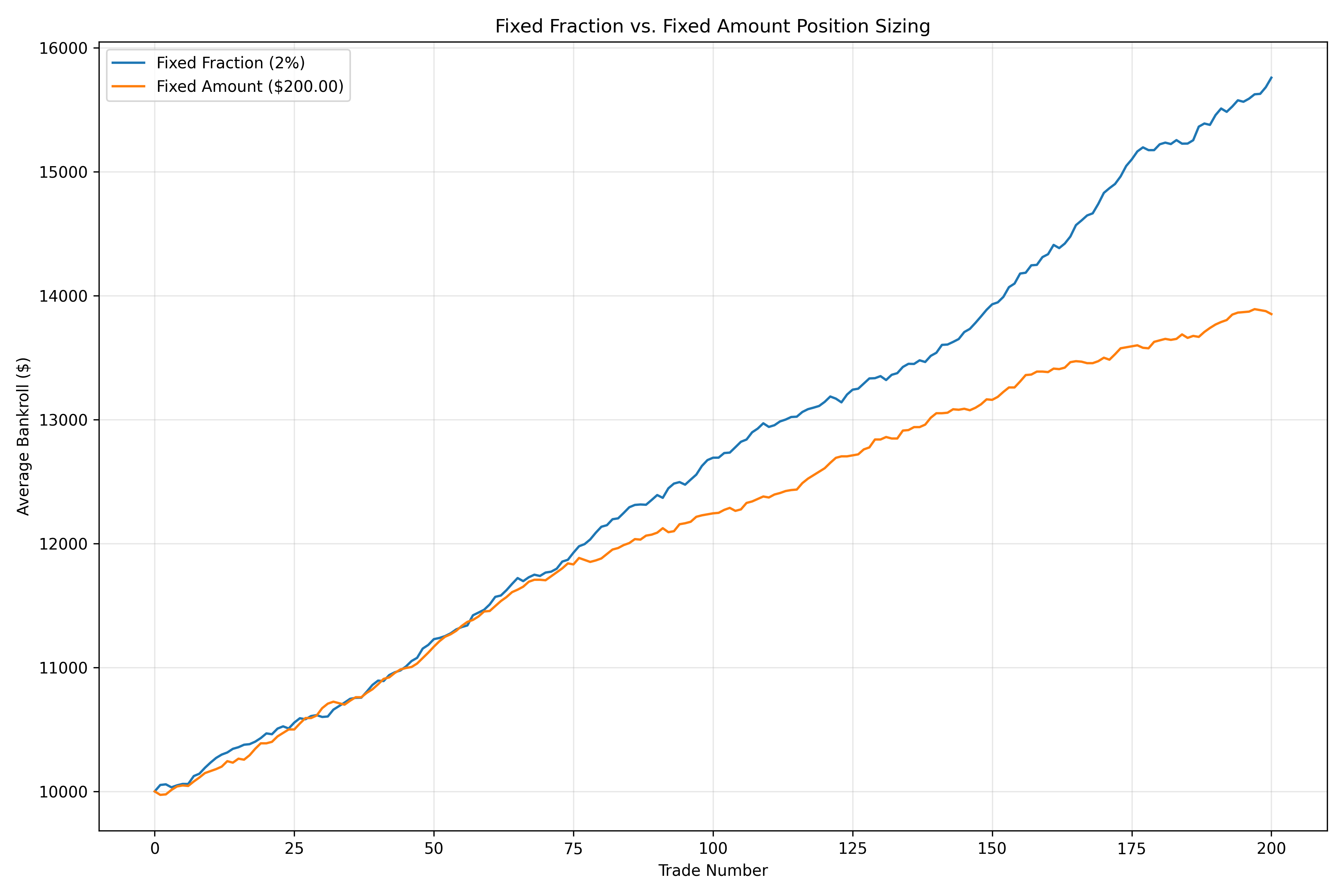
The chart above illustrates how bet amounts change with different fixed fractions as your bankroll grows. Notice that higher fractions lead to larger bets but also greater risk.

The Theory Behind Fixed Fraction

The mathematical foundation of the Fixed Fraction strategy is straightforward:

Bet amount = f * Current bankroll

Where f is the fixed fraction you choose (e.g., 0.01 for 1%, 0.02 for 2%, etc.).

This creates a natural scaling mechanism: as your bankroll grows, your bet sizes increase; as it shrinks, your bet sizes decrease. This automatic adjustment helps protect your bankroll during losing streaks while allowing you to capitalize on winning streaks.

Pros of Fixed Fraction

Simplicity: Extremely easy to understand and implement
No probability estimates needed: Works without knowing your exact edge
Automatic scaling: Naturally adjusts bet sizes as your bankroll changes
Prevents ruin: Theoretically impossible to go completely broke (though you can get very close)
Psychological comfort: Consistent approach regardless of recent results

Cons of Fixed Fraction

Not mathematically optimal: Doesn’t maximize long-term growth like Kelly
Ignores your edge: Same bet size regardless of how good the opportunity is
Can be too conservative: Often leaves money on the table with strong edges
Can be too aggressive: May bet too much when you have minimal edge
Slow recovery: Can take a long time to recover from significant drawdowns

Implementing Fixed Fraction with Keeks

Using the Fixed Fraction strategy with Keeks is straightforward:

from keeks.bankroll import BankRoll
from keeks.binary_strategies.fixed_fraction import FixedFraction
from keeks.simulators.repeated_binary import RepeatedBinarySimulator
import matplotlib.pyplot as plt

# Create a bankroll with initial funds
bankroll = BankRoll(initial_funds=1000.0)

# Create a Fixed Fraction strategy with 2% risk per bet
fixed_fraction = FixedFraction(fraction=0.02)

# Calculate the bet amount for our current bankroll
bet_amount = fixed_fraction.calculate_bet_amount(bankroll.current_funds)
print(f"Initial bankroll: ${bankroll.current_funds:.2f}")
print(f"Fixed fraction: {fixed_fraction.fraction:.2%}")
print(f"Initial bet amount: ${bet_amount:.2f}")

# Simulate 1000 bets using Fixed Fraction
# Let's assume we have a 55% chance of winning with even money payouts
simulator = RepeatedBinarySimulator(
    payoff=1.0, 
    loss=1.0, 
    probability=0.55,
    trials=1000
)

# Run the simulation
simulator.evaluate_strategy(fixed_fraction, bankroll)

# Plot the results
plt.figure(figsize=(10, 6))
plt.plot(bankroll.history)
plt.title('Bankroll Growth Using Fixed Fraction (2%)')
plt.xlabel('Number of Bets')
plt.ylabel('Bankroll Size')
plt.grid(True)
plt.show()

# Print final results
final_bankroll = bankroll.history[-1]
growth_rate = (final_bankroll / 1000.0) ** (1 / 1000) - 1
print(f"Final bankroll: ${final_bankroll:.2f}")
print(f"Growth rate: {growth_rate:.2%} per bet")

Bankroll Over Time

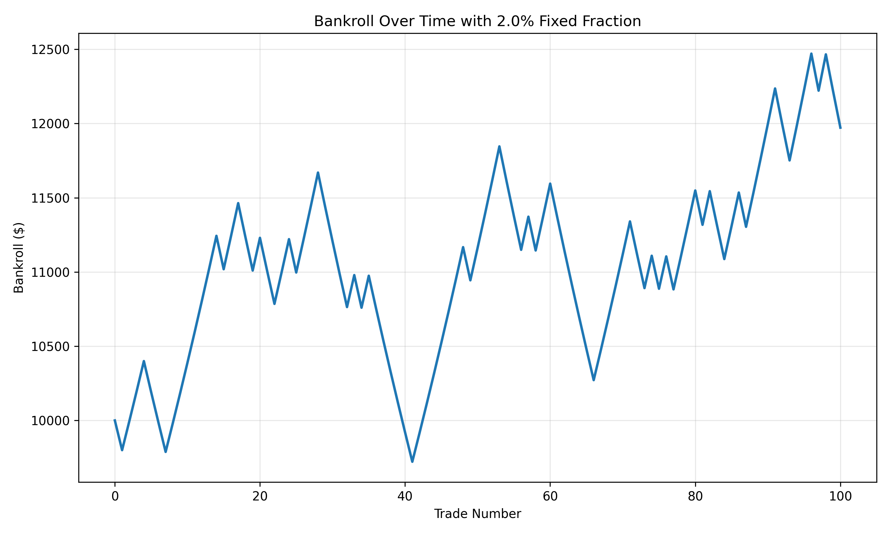
The chart above shows how a bankroll evolves over time using the Fixed Fraction strategy with a 2% fraction. Notice the steady growth with occasional drawdowns.

Comparing Different Fixed Fractions

Let’s compare how different fixed fractions perform over time:

import numpy as np
from keeks.bankroll import BankRoll
from keeks.binary_strategies.fixed_fraction import FixedFraction
from keeks.simulators.repeated_binary import RepeatedBinarySimulator
import matplotlib.pyplot as plt

# Set up simulation parameters
initial_funds = 1000.0
win_probability = 0.55
payoff = 1.0
loss = 1.0
trials = 1000
num_simulations = 100

# Fractions to compare
fractions = [0.01, 0.02, 0.05, 0.10, 0.25]

# Store results
results = {}

for fraction in fractions:
    # Run multiple simulations for this fraction
    final_bankrolls = []
    
    for _ in range(num_simulations):
        bankroll = BankRoll(initial_funds=initial_funds)
        strategy = FixedFraction(fraction=fraction)
        
        simulator = RepeatedBinarySimulator(
            payoff=payoff,
            loss=loss,
            probability=win_probability,
            trials=trials
        )
        
        simulator.evaluate_strategy(strategy, bankroll)
        final_bankrolls.append(bankroll.history[-1])
    
    # Calculate statistics
    avg_final = np.mean(final_bankrolls)
    median_final = np.median(final_bankrolls)
    min_final = np.min(final_bankrolls)
    max_final = np.max(final_bankrolls)
    
    # Calculate average growth rate
    avg_growth_rate = (avg_final / initial_funds) ** (1 / trials) - 1
    
    results[fraction] = {
        'avg_final': avg_final,
        'median_final': median_final,
        'min_final': min_final,
        'max_final': max_final,
        'avg_growth_rate': avg_growth_rate
    }
    
    print(f"Fixed Fraction {fraction:.2%}:")
    print(f"  Average final bankroll: ${avg_final:.2f}")
    print(f"  Average growth rate: {avg_growth_rate:.4%} per bet")
    print(f"  Range: ${min_final:.2f} to ${max_final:.2f}")
    print()

# Plot average final bankrolls
plt.figure(figsize=(10, 6))
fractions_pct = [f * 100 for f in fractions]
avg_finals = [results[f]['avg_final'] for f in fractions]

plt.bar(fractions_pct, avg_finals)
plt.title('Average Final Bankroll by Fixed Fraction')
plt.xlabel('Fixed Fraction (%)')
plt.ylabel('Average Final Bankroll ($)')
plt.grid(True, axis='y')
plt.show()

Average Bankroll Comparison

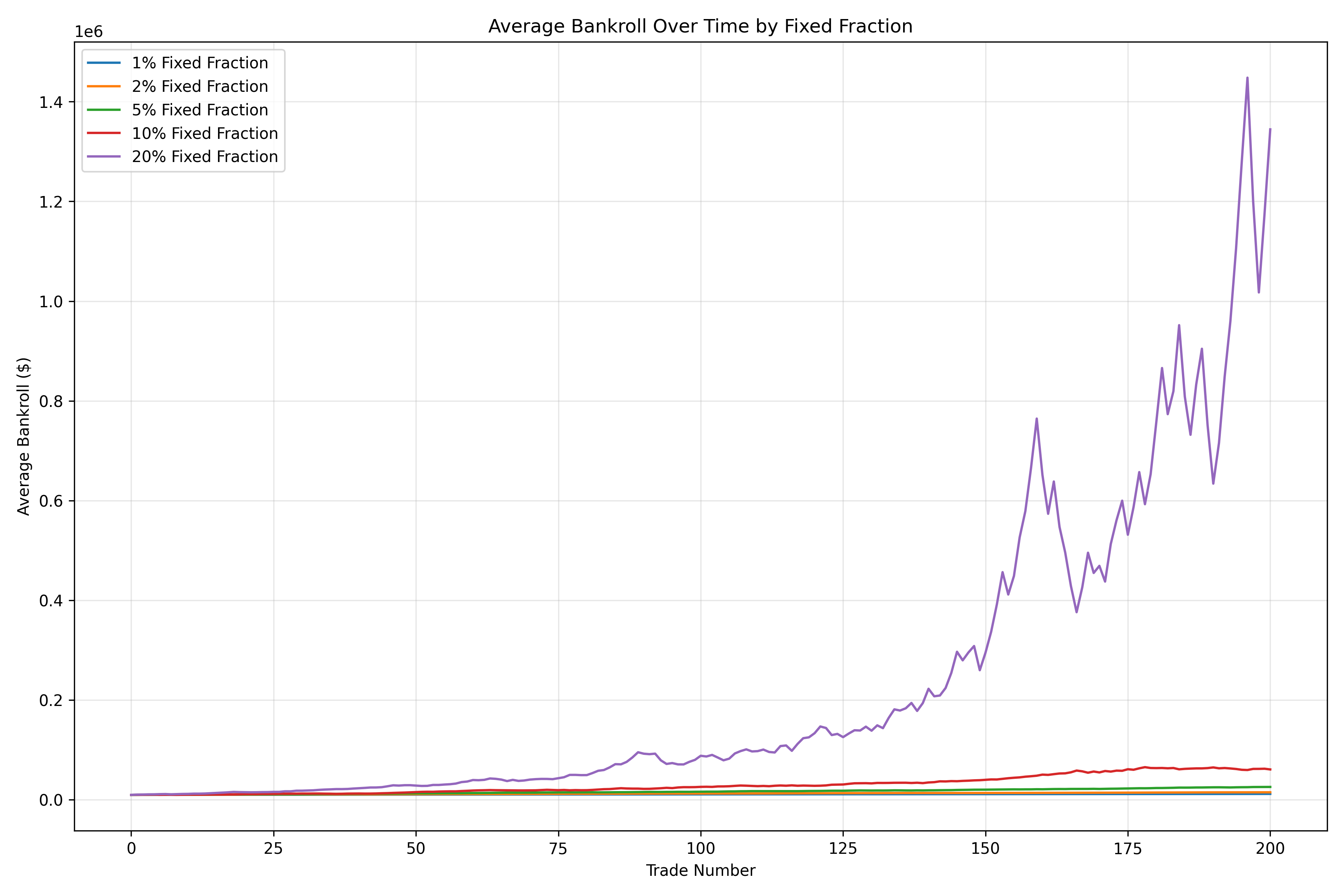
This chart compares the average final bankroll for different fixed fractions. Notice that there’s an optimal fraction that balances growth and risk.

Final Bankroll Distribution

The distribution of final bankrolls shows how different fixed fractions affect the range of possible outcomes. Higher fractions lead to wider distributions with both higher potential gains and deeper potential losses.

Finding the Optimal Fixed Fraction

While the Fixed Fraction strategy doesn’t aim to be mathematically optimal like Kelly, we can still find the fraction that performs best for a given scenario:

import numpy as np
from keeks.bankroll import BankRoll
from keeks.binary_strategies.fixed_fraction import FixedFraction
from keeks.simulators.repeated_binary import RepeatedBinarySimulator
import matplotlib.pyplot as plt

# Set up simulation parameters
initial_funds = 1000.0
win_probability = 0.55
payoff = 1.0
loss = 1.0
trials = 1000
num_simulations = 50

# Fractions to test
fractions = np.linspace(0.01, 0.5, 50)

# Store results
avg_finals = []
avg_growth_rates = []

for fraction in fractions:
    # Run multiple simulations for this fraction
    final_bankrolls = []
    
    for _ in range(num_simulations):
        bankroll = BankRoll(initial_funds=initial_funds)
        strategy = FixedFraction(fraction=fraction)
        
        simulator = RepeatedBinarySimulator(
            payoff=payoff,
            loss=loss,
            probability=win_probability,
            trials=trials
        )
        
        simulator.evaluate_strategy(strategy, bankroll)
        final_bankrolls.append(bankroll.history[-1])
    
    # Calculate average final bankroll
    avg_final = np.mean(final_bankrolls)
    avg_finals.append(avg_final)
    
    # Calculate average growth rate
    avg_growth_rate = (avg_final / initial_funds) ** (1 / trials) - 1
    avg_growth_rates.append(avg_growth_rate)

# Find the optimal fraction
optimal_idx = np.argmax(avg_finals)
optimal_fraction = fractions[optimal_idx]
optimal_final = avg_finals[optimal_idx]
optimal_growth_rate = avg_growth_rates[optimal_idx]

print(f"Optimal fixed fraction: {optimal_fraction:.2%}")
print(f"Average final bankroll: ${optimal_final:.2f}")
print(f"Average growth rate: {optimal_growth_rate:.4%} per bet")

# Plot the results
plt.figure(figsize=(10, 6))
plt.plot(fractions * 100, avg_finals)
plt.axvline(x=optimal_fraction * 100, color='r', linestyle='--', 
            label=f'Optimal: {optimal_fraction:.2%}')
plt.title('Average Final Bankroll by Fixed Fraction')
plt.xlabel('Fixed Fraction (%)')
plt.ylabel('Average Final Bankroll ($)')
plt.grid(True)
plt.legend()
plt.show()

EV vs Fraction

This chart shows how the expected value (average final bankroll) changes with different fixed fractions. The optimal fraction maximizes the expected value.

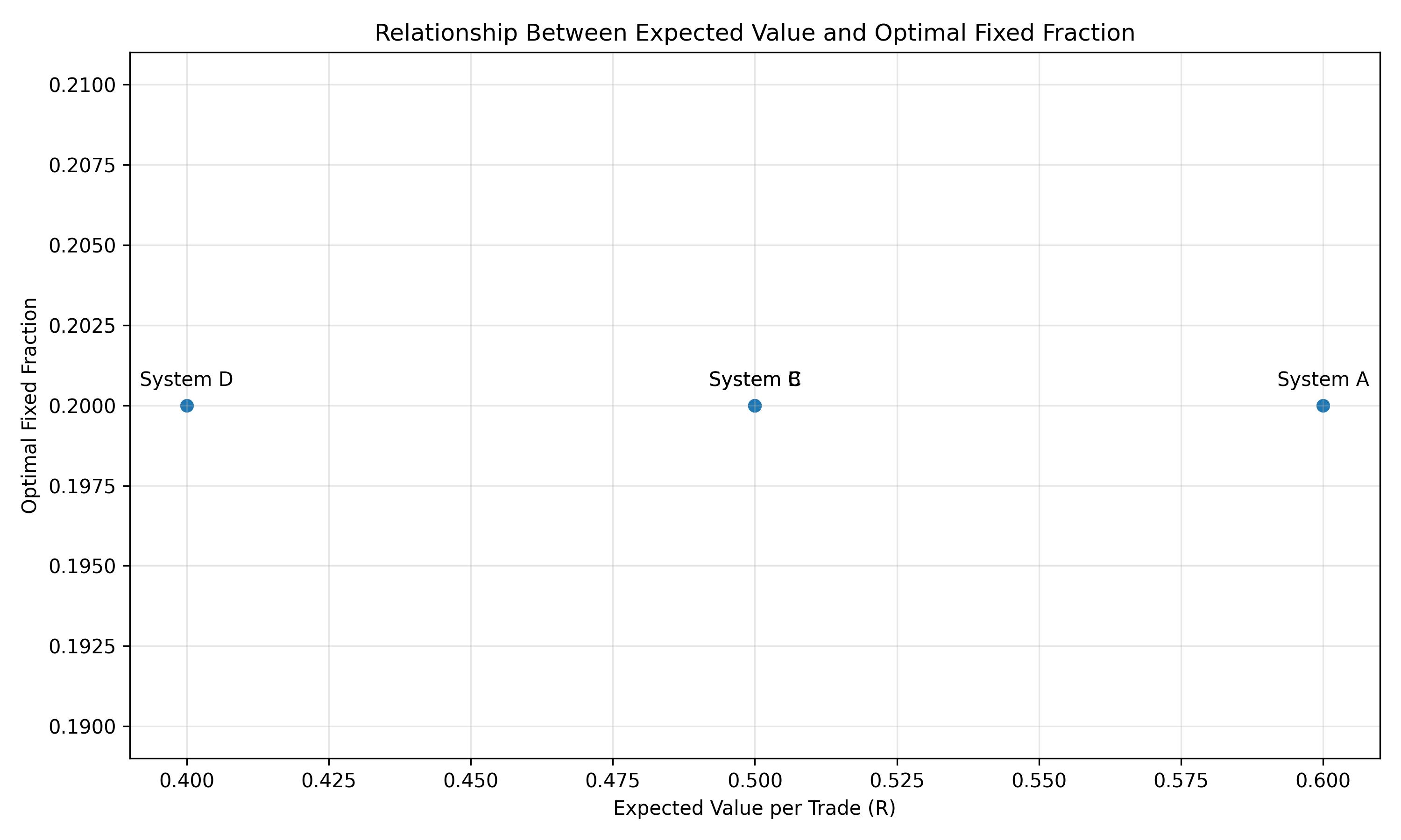
Optimal Fixed Fractions for Different Scenarios

The optimal fixed fraction depends on your edge (win probability and payoff ratio). Let’s explore how it changes across different scenarios:

import numpy as np
import matplotlib.pyplot as plt
from keeks.bankroll import BankRoll
from keeks.binary_strategies.fixed_fraction import FixedFraction
from keeks.simulators.repeated_binary import RepeatedBinarySimulator

# Set up simulation parameters
initial_funds = 1000.0
trials = 500
num_simulations = 30
fractions = np.linspace(0.01, 0.5, 25)

# Scenarios to test
scenarios = [
    {"win_prob": 0.52, "payoff": 1.0, "loss": 1.0, "label": "52% win, 1:1 odds"},
    {"win_prob": 0.55, "payoff": 1.0, "loss": 1.0, "label": "55% win, 1:1 odds"},
    {"win_prob": 0.60, "payoff": 1.0, "loss": 1.0, "label": "60% win, 1:1 odds"},
    {"win_prob": 0.40, "payoff": 2.0, "loss": 1.0, "label": "40% win, 2:1 odds"},
    {"win_prob": 0.33, "payoff": 3.0, "loss": 1.0, "label": "33% win, 3:1 odds"}
]

# Store results
optimal_fractions = {}

for scenario in scenarios:
    win_prob = scenario["win_prob"]
    payoff = scenario["payoff"]
    loss = scenario["loss"]
    label = scenario["label"]
    
    avg_finals = []
    
    for fraction in fractions:
        # Run multiple simulations for this fraction
        final_bankrolls = []
        
        for _ in range(num_simulations):
            bankroll = BankRoll(initial_funds=initial_funds)
            strategy = FixedFraction(fraction=fraction)
            
            simulator = RepeatedBinarySimulator(
                payoff=payoff,
                loss=loss,
                probability=win_prob,
                trials=trials
            )
            
            simulator.evaluate_strategy(strategy, bankroll)
            final_bankrolls.append(bankroll.history[-1])
        
        # Calculate average final bankroll
        avg_final = np.mean(final_bankrolls)
        avg_finals.append(avg_final)
    
    # Find the optimal fraction
    optimal_idx = np.argmax(avg_finals)
    optimal_fraction = fractions[optimal_idx]
    optimal_final = avg_finals[optimal_idx]
    
    optimal_fractions[label] = {
        "fraction": optimal_fraction,
        "avg_final": optimal_final,
        "win_prob": win_prob,
        "payoff": payoff,
        "loss": loss
    }
    
    print(f"Scenario: {label}")
    print(f"  Optimal fixed fraction: {optimal_fraction:.2%}")
    print(f"  Average final bankroll: ${optimal_final:.2f}")
    print()

# Calculate Kelly fractions for comparison
kelly_fractions = {}
for label, data in optimal_fractions.items():
    p = data["win_prob"]
    b = data["payoff"] / data["loss"]
    kelly = p - (1-p)/b
    kelly_fractions[label] = kelly
    
    print(f"Scenario: {label}")
    print(f"  Optimal fixed fraction: {data['fraction']:.2%}")
    print(f"  Kelly fraction: {kelly:.2%}")
    print(f"  Ratio (Optimal/Kelly): {data['fraction']/kelly:.2f}")
    print()

# Plot the results
plt.figure(figsize=(12, 8))
labels = list(optimal_fractions.keys())
opt_fracs = [optimal_fractions[label]["fraction"] for label in labels]
kelly_fracs = [kelly_fractions[label] for label in labels]

x = np.arange(len(labels))
width = 0.35

plt.bar(x - width/2, [f * 100 for f in opt_fracs], width, label='Optimal Fixed Fraction')
plt.bar(x + width/2, [f * 100 for f in kelly_fracs], width, label='Kelly Fraction')

plt.ylabel('Fraction (%)')
plt.title('Optimal Fixed Fraction vs Kelly Fraction')
plt.xticks(x, labels, rotation=45, ha='right')
plt.legend()
plt.tight_layout()
plt.grid(True, axis='y')
plt.show()

Optimal Fractions

This chart compares the optimal fixed fractions with Kelly fractions across different scenarios. Notice that the optimal fixed fraction is typically lower than the Kelly fraction, reflecting the more conservative nature of the Fixed Fraction strategy.

Practical Applications of Fixed Fraction

The Fixed Fraction strategy is widely used in various domains:

1. Sports Betting

Fixed Fraction is popular among sports bettors due to its simplicity. For example, a bettor with a $1,000 bankroll using a 2% fixed fraction would bet $20 on their first wager. If they win and their bankroll grows to $1,020, their next bet would be $20.40 (2% of $1,020).

2. Trading and Investing

Many traders use a fixed percentage of their portfolio for each position. For instance, a trader might allocate 1% of their capital to each trade, automatically scaling position sizes as their account grows or shrinks.

3. Poker Bankroll Management

Poker players often use fixed fraction rules for moving up or down in stakes. A common rule is the “20 buy-in rule,” where players maintain at least 20 buy-ins for their current stake level.

When to Use Fixed Fraction

Fixed Fraction is particularly well-suited for:

Beginners: The simplicity makes it ideal for those new to bankroll management
Uncertain edges: When you don’t have reliable probability estimates
Psychological comfort: When you prefer consistency over optimization
Multiple bet types: When dealing with various bet types with different edges
Long-term sustainability: When capital preservation is a priority

Practical Recommendations

Based on both theory and empirical evidence, here are some practical recommendations for using the Fixed Fraction strategy:

Start conservative: Begin with a small fraction (1-2%) until you gain confidence in your edge.
Adjust based on edge: Use larger fractions (3-5%) when you have a strong edge, smaller fractions (0.5-1%) when your edge is minimal.
Consider your risk tolerance: Higher fractions lead to higher volatility. Choose a fraction that allows you to sleep at night.
Periodically reassess: Review your results and adjust your fraction as needed.
Combine with other methods: Consider using Fixed Fraction as a maximum bet size, even when other methods suggest larger bets.

Conclusion

The Fixed Fraction strategy offers a simple yet effective approach to bankroll management. While it may not maximize growth like Kelly-based methods, its simplicity, consistency, and built-in risk management make it a popular choice for many bettors, traders, and investors.

By choosing an appropriate fraction based on your edge and risk tolerance, you can achieve steady growth while protecting your bankroll from devastating losses. The automatic scaling of bet sizes provides a natural balance between aggression and caution.

In our next post, we’ll explore the Constant Proportion Portfolio Insurance (CPPI) strategy, which combines elements of fixed fraction with downside protection.