Bankroll Management with Keeks: CPPI
In our previous posts, we’ve explored various bankroll management strategies, from the mathematically optimal Kelly Criterion to the straightforward Fixed Fraction approach. Today, we’ll examine a strategy that prioritizes capital preservation: Constant Proportion Portfolio Insurance (CPPI).
What is CPPI?
Constant Proportion Portfolio Insurance (CPPI) is a dynamic asset allocation strategy that aims to provide downside protection while still allowing for upside participation. Developed by Fischer Black and André Perold in the 1980s for portfolio management, CPPI can be adapted for bankroll management in betting and trading.
The core idea is simple: protect a predetermined “floor” value of your bankroll while investing a multiple of the excess capital (the “cushion”) in risky bets or investments.
The Theory Behind CPPI
The CPPI formula determines how much to bet or invest:
Bet amount = m * (Current bankroll - Floor)
Where:
mis the multiplier (typically between 1 and 5)Flooris the minimum bankroll value you want to protectCurrent bankroll - Flooris the cushion
As your bankroll grows, the cushion increases, allowing for larger bets. If your bankroll shrinks and approaches the floor, bet sizes automatically decrease to protect your capital. If your bankroll ever reaches the floor value, betting stops entirely until the bankroll increases again.
Pros of CPPI
- Capital preservation: Protects a minimum bankroll value
- Downside protection: Automatically reduces exposure during drawdowns
- Customizable risk: Adjustable floor and multiplier based on risk tolerance
- Psychological comfort: Knowing you won’t lose below a certain amount
- Participation in upside: Still allows for growth when performing well
Cons of CPPI
- Opportunity cost: Less aggressive than Kelly or Fixed Fraction when winning
- Parameter sensitivity: Results heavily depend on floor and multiplier choices
- Cash drag: The floor portion effectively earns zero return
- Not mathematically optimal: Doesn’t maximize long-term growth
- Gap risk: Sudden large losses can breach the floor
Implementing CPPI with Keeks
Using CPPI with Keeks is straightforward:
from keeks.bankroll import BankRoll
from keeks.binary_strategies.cppi import CPPI
from keeks.simulators.repeated_binary import RepeatedBinarySimulator
import matplotlib.pyplot as plt

# Create a bankroll with initial funds
initial_funds = 1000.0
bankroll = BankRoll(initial_funds=initial_funds)

# Create a CPPI strategy
# Floor is 80% of initial bankroll, multiplier is 3
floor = 0.8 * initial_funds
multiplier = 3
cppi = CPPI(floor=floor, multiplier=multiplier)

# Calculate the initial bet amount
cushion = bankroll.current_funds - floor
bet_amount = cppi.calculate_bet_amount(bankroll.current_funds)

print(f"Initial bankroll: ${bankroll.current_funds:.2f}")
print(f"Floor: ${floor:.2f}")
print(f"Cushion: ${cushion:.2f}")
print(f"Multiplier: {multiplier}")
print(f"Initial bet amount: ${bet_amount:.2f}")
print(f"Bet as percentage of bankroll: {bet_amount/bankroll.current_funds:.2%}")

# Simulate 1000 bets using CPPI
# Let's assume we have a 55% chance of winning with even money payouts
simulator = RepeatedBinarySimulator(
    payoff=1.0,
    loss=1.0,
    probability=0.55,
    trials=1000
)

# Run the simulation
simulator.evaluate_strategy(cppi, bankroll)

# Plot the results
plt.figure(figsize=(10, 6))
plt.plot(bankroll.history)
plt.axhline(y=floor, color='r', linestyle='--', label='Floor')
plt.title('Bankroll Growth Using CPPI')
plt.xlabel('Number of Bets')
plt.ylabel('Bankroll Size')
plt.legend()
plt.grid(True)
plt.show()

# Print final results
final_bankroll = bankroll.history[-1]
growth_rate = (final_bankroll / initial_funds) ** (1 / 1000) - 1
print(f"Final bankroll: ${final_bankroll:.2f}")
print(f"Growth rate: {growth_rate:.2%} per bet")
print(f"Minimum bankroll: ${min(bankroll.history):.2f}")
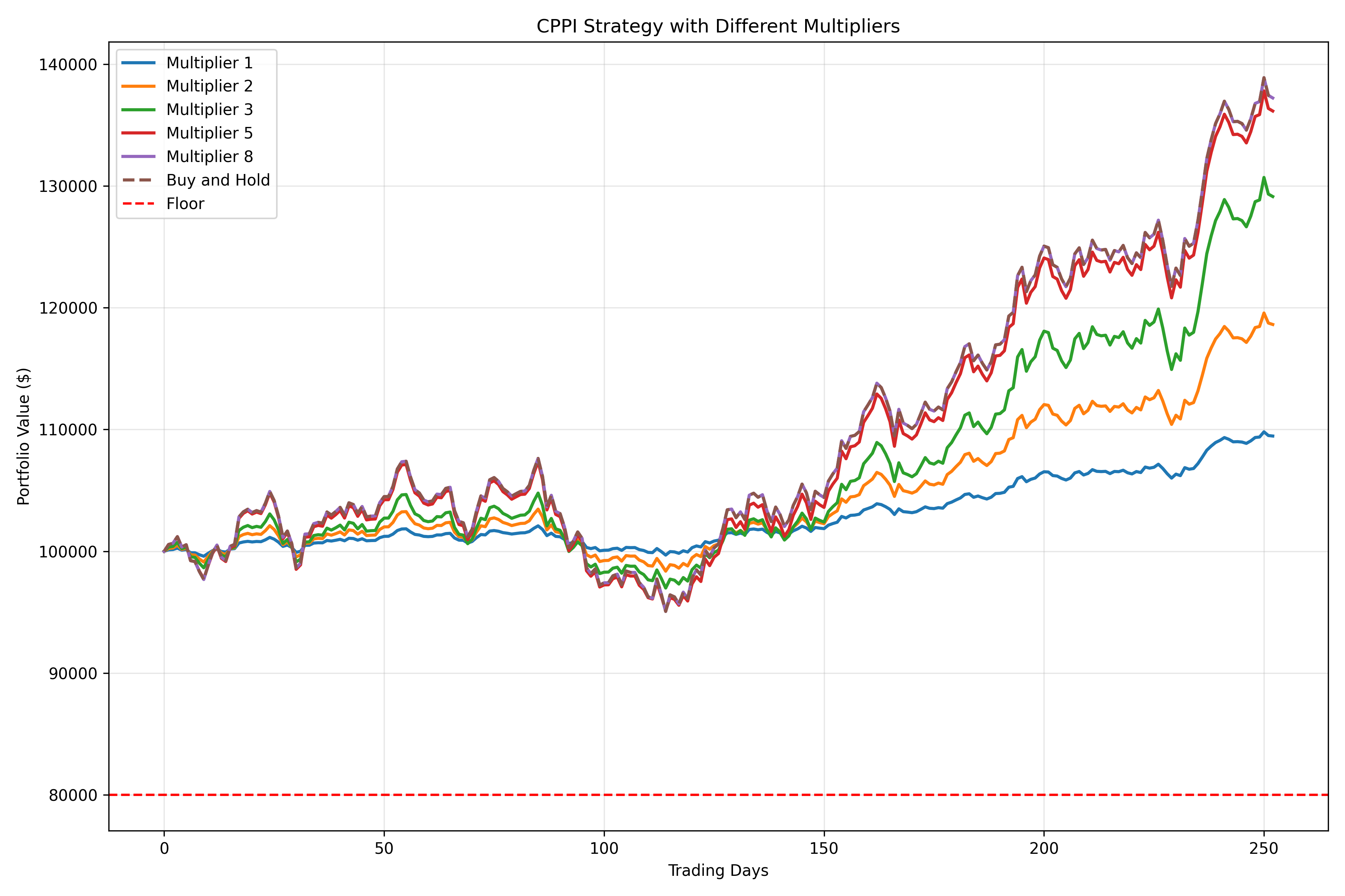
Exploring Different CPPI Parameters
Let’s compare how different floor levels and multipliers affect performance:
import numpy as np
from keeks.bankroll import BankRoll
from keeks.binary_strategies.cppi import CPPI
from keeks.simulators.repeated_binary import RepeatedBinarySimulator
import matplotlib.pyplot as plt

# Set up our simulation parameters
win_probability = 0.55
payoff = 1.0
loss = 1.0
trials = 1000
initial_funds = 1000.0

# Create strategies with different CPPI parameters
strategies = {
    "Conservative (Floor: 90%, m=2)": CPPI(floor=0.9*initial_funds, multiplier=2),
    "Moderate (Floor: 80%, m=3)": CPPI(floor=0.8*initial_funds, multiplier=3),
    "Aggressive (Floor: 70%, m=4)": CPPI(floor=0.7*initial_funds, multiplier=4),
    "Very Aggressive (Floor: 60%, m=5)": CPPI(floor=0.6*initial_funds, multiplier=5)
}

# Create a simulator with fixed random seed for fair comparison
simulator = RepeatedBinarySimulator(
    payoff=payoff,
    loss=loss,
    probability=win_probability,
    trials=trials,
    random_seed=42  # Fixed seed ensures same sequence of wins/losses
)

# Run simulations
results = {}

for name, strategy in strategies.items():
    bankroll = BankRoll(initial_funds=initial_funds)
    simulator.evaluate_strategy(strategy, bankroll)
    results[name] = {
        "history": bankroll.history.copy(),
        "drawdowns": bankroll.drawdown_history.copy(),
        "floor": strategy.floor
    }

# Plot the bankroll histories
plt.figure(figsize=(12, 8))
for name, data in results.items():
    plt.plot(data["history"], label=name)
    plt.axhline(y=data["floor"], color=plt.gca().lines[-1].get_color(), linestyle='--', alpha=0.3)

plt.title('Comparison of CPPI Strategies')
plt.xlabel('Number of Bets')
plt.ylabel('Bankroll Size')
plt.legend()
plt.grid(True)
plt.show()

# Calculate and display statistics
for name, data in results.items():
    history = data["history"]
    drawdowns = data["drawdowns"]
    floor = data["floor"]

    final_value = history[-1]
    min_value = min(history)
    max_drawdown = max(drawdowns) * 100
    growth_rate = (final_value / initial_funds) ** (1 / trials) - 1
    min_cushion = min_value - floor

    print(f"{name}:")
    print(f"  Final bankroll: ${final_value:.2f}")
    print(f"  Growth rate: {growth_rate:.2%} per bet")
    print(f"  Minimum bankroll: ${min_value:.2f}")
    print(f"  Minimum cushion: ${min_cushion:.2f}")
    print(f"  Maximum drawdown: {max_drawdown:.2f}%")
    print()
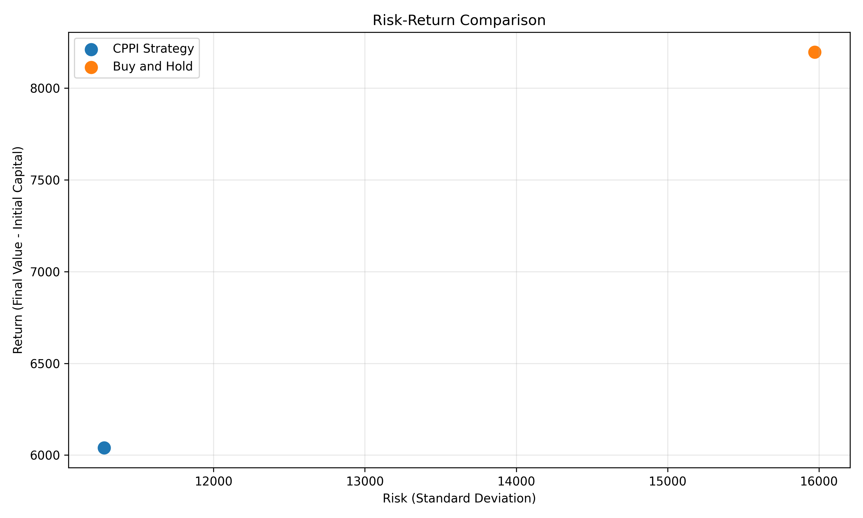
Comparing CPPI with Other Strategies
Let’s see how CPPI compares to Kelly and Fixed Fraction strategies:
from keeks.bankroll import BankRoll
from keeks.binary_strategies.kelly import KellyCriterion
from keeks.binary_strategies.fixed_fraction import FixedFraction
from keeks.binary_strategies.cppi import CPPI
from keeks.simulators.repeated_binary import RepeatedBinarySimulator
import matplotlib.pyplot as plt

# Set up our simulation parameters
win_probability = 0.55
payoff = 1.0
loss = 1.0
trials = 1000
initial_funds = 1000.0

# Create strategies
kelly = KellyCriterion(payoff=payoff, loss=loss)
fixed_fraction = FixedFraction(fraction=0.05)
cppi_conservative = CPPI(floor=0.9*initial_funds, multiplier=3)
cppi_aggressive = CPPI(floor=0.7*initial_funds, multiplier=4)

# Create a simulator with fixed random seed for fair comparison
simulator = RepeatedBinarySimulator(
    payoff=payoff,
    loss=loss,
    probability=win_probability,
    trials=trials,
    random_seed=42  # Fixed seed ensures same sequence of wins/losses
)

# Run simulations
results = {}
strategies = {
    "Kelly": kelly,
    "Fixed Fraction (5%)": fixed_fraction,
    "CPPI Conservative": cppi_conservative,
    "CPPI Aggressive": cppi_aggressive
}

for name, strategy in strategies.items():
    bankroll = BankRoll(initial_funds=initial_funds)
    simulator.evaluate_strategy(strategy, bankroll)
    results[name] = {
        "history": bankroll.history.copy(),
        "drawdowns": bankroll.drawdown_history.copy(),
        "floor": getattr(strategy, 'floor', 0)  # Only CPPI has a floor
    }

# Plot the bankroll histories
plt.figure(figsize=(12, 8))
for name, data in results.items():
    plt.plot(data["history"], label=name)
    if data["floor"] > 0:
        plt.axhline(y=data["floor"], color=plt.gca().lines[-1].get_color(), linestyle='--', alpha=0.3)

plt.title('CPPI vs Other Strategies')
plt.xlabel('Number of Bets')
plt.ylabel('Bankroll Size')
plt.legend()
plt.grid(True)
plt.show()

# Plot the drawdown histories
plt.figure(figsize=(12, 8))
for name, data in results.items():
    plt.plot(data["drawdowns"], label=name)

plt.title('Drawdown Comparison')
plt.xlabel('Number of Bets')
plt.ylabel('Drawdown (%)')
plt.legend()
plt.grid(True)
plt.show()

# Calculate and display statistics
for name, data in results.items():
    history = data["history"]
    drawdowns = data["drawdowns"]

    final_value = history[-1]
    min_value = min(history)
    max_drawdown = max(drawdowns) * 100
    growth_rate = (final_value / initial_funds) ** (1 / trials) - 1

    print(f"{name}:")
    print(f"  Final bankroll: ${final_value:.2f}")
    print(f"  Growth rate: {growth_rate:.2%} per bet")
    print(f"  Minimum bankroll: ${min_value:.2f}")
    print(f"  Maximum drawdown: {max_drawdown:.2f}%")
    print()
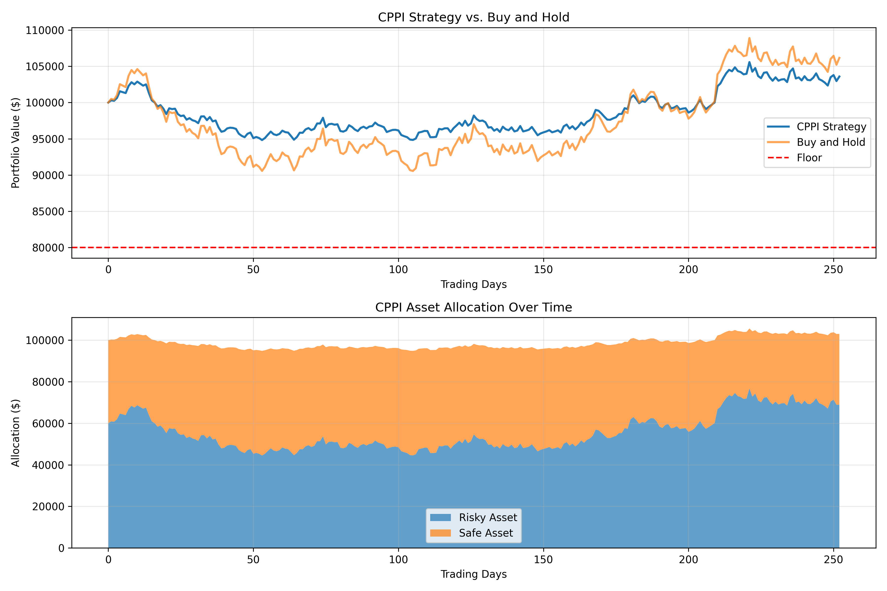
Real-World Example: Investment Portfolio Protection
Let’s consider a practical example of using CPPI for an investment portfolio:
from keeks.bankroll import BankRoll
from keeks.binary_strategies.cppi import CPPI
import numpy as np
import matplotlib.pyplot as plt

# Create a portfolio with $100,000
initial_capital = 100000.0
portfolio = BankRoll(initial_funds=initial_capital)

# Let's say we want to protect 90% of our initial capital
floor = 0.9 * initial_capital  # $90,000
multiplier = 3

# Create a CPPI strategy
cppi = CPPI(floor=floor, multiplier=multiplier)

# Calculate initial allocation
initial_cushion = initial_capital - floor
initial_risky_allocation = cppi.calculate_bet_amount(initial_capital)
initial_safe_allocation = initial_capital - initial_risky_allocation

print(f"Initial portfolio: ${initial_capital:.2f}")
print(f"Floor: ${floor:.2f}")
print(f"Initial cushion: ${initial_cushion:.2f}")
print(f"Initial risky allocation: ${initial_risky_allocation:.2f} ({initial_risky_allocation/initial_capital:.2%})")
print(f"Initial safe allocation: ${initial_safe_allocation:.2f} ({initial_safe_allocation/initial_capital:.2%})")

# Let's simulate a market scenario with some volatility
# We'll use monthly returns for a year
np.random.seed(42)
months = 12
monthly_returns = np.random.normal(0.01, 0.05, months)  # Mean 1%, std dev 5%

# Track our allocations over time
portfolio_values = [initial_capital]
risky_allocations = [initial_risky_allocation]
safe_allocations = [initial_safe_allocation]
cushions = [initial_cushion]

# Simulate the portfolio over time
current_value = initial_capital
for i, monthly_return in enumerate(monthly_returns):
    # Calculate return on the risky portion
    risky_allocation = risky_allocations[-1]
    safe_allocation = safe_allocations[-1]

    # Update portfolio value
    risky_return = risky_allocation * monthly_return
    current_value += risky_return

    # Rebalance using CPPI
    new_risky_allocation = cppi.calculate_bet_amount(current_value)
    new_safe_allocation = current_value - new_risky_allocation
    new_cushion = current_value - floor

    # Record values
    portfolio_values.append(current_value)
    risky_allocations.append(new_risky_allocation)
    safe_allocations.append(new_safe_allocation)
    cushions.append(new_cushion)

    print(f"Month {i+1}: Return: {monthly_return:.2%}, Portfolio: ${current_value:.2f}, Risky: ${new_risky_allocation:.2f} ({new_risky_allocation/current_value:.2%})")

# Plot the results
plt.figure(figsize=(12, 8))
plt.subplot(2, 1, 1)
plt.plot(portfolio_values, label='Portfolio Value')
plt.axhline(y=floor, color='r', linestyle='--', label='Floor')
plt.title('Portfolio Value Over Time')
plt.legend()
plt.grid(True)

plt.subplot(2, 1, 2)
plt.plot(risky_allocations, label='Risky Allocation')
plt.plot(safe_allocations, label='Safe Allocation')
plt.title('Asset Allocation Over Time')
plt.legend()
plt.grid(True)

plt.tight_layout()
plt.show()

# Calculate final statistics
final_value = portfolio_values[-1]
min_value = min(portfolio_values)
max_drawdown = (max(portfolio_values) - min(portfolio_values)) / max(portfolio_values) * 100
total_return = (final_value / initial_capital - 1) * 100

print(f"\nFinal Statistics:")
print(f"  Final portfolio value: ${final_value:.2f}")
print(f"  Total return: {total_return:.2f}%")
print(f"  Minimum portfolio value: ${min_value:.2f}")
print(f"  Maximum drawdown: {max_drawdown:.2f}%")
When to Use CPPI
CPPI is particularly well-suited for:
- Capital preservation: When protecting a minimum bankroll is critical
- Retirement planning: When you can’t afford to lose below a certain amount
- Goal-based investing: When saving for specific financial goals
- Risk-averse bettors: Who want downside protection with upside potential
- Recovery situations: When rebuilding after significant losses
Choosing Your CPPI Parameters
The key parameters in CPPI are the floor and multiplier:
Floor Selection
- Higher floor (e.g., 90%): More conservative, greater capital protection
- Medium floor (e.g., 80%): Balanced approach
- Lower floor (e.g., 70%): More aggressive, allows for more risk-taking
Multiplier Selection
- Lower multiplier (e.g., 2): More conservative, slower growth
- Medium multiplier (e.g., 3-4): Balanced approach
- Higher multiplier (e.g., 5+): More aggressive, faster growth but higher risk
The optimal combination depends on your risk tolerance, investment horizon, and financial goals.
Conclusion
Constant Proportion Portfolio Insurance (CPPI) offers a unique approach to bankroll management that prioritizes capital preservation while still allowing for growth. By dynamically adjusting exposure based on the cushion above your floor value, CPPI provides a systematic way to protect your downside while participating in upside potential.
While not mathematically optimal for maximum growth, CPPI’s focus on protecting a minimum bankroll value makes it an attractive option for risk-averse bettors and investors, or for those with specific financial goals they can’t afford to miss.
In our next post, we’ll explore Dynamic Bankroll Management, an adaptive strategy that adjusts bet sizing based on recent performance and market conditions.
Stay in the loop
Get notified when I publish new posts. No spam, unsubscribe anytime.