Bankroll Management with Keeks: Dynamic Strategies
In our previous posts, we’ve explored various bankroll management strategies, from the mathematically optimal Kelly Criterion to the capital-preserving CPPI. Today, we’ll examine Dynamic Bankroll Management, an adaptive approach that adjusts bet sizing based on recent performance and market conditions.
What is Dynamic Bankroll Management?
Dynamic Bankroll Management (DBM) is a flexible strategy that modifies your bet sizing based on various factors that change over time, such as:
- Recent performance (winning or losing streaks)
- Volatility in your results
- Changes in your edge or confidence
- Market conditions or opportunities
Unlike static strategies that apply the same formula regardless of circumstances, DBM adapts to the evolving landscape of your betting or investing environment.
The Theory Behind Dynamic Bankroll Management
The core principle of DBM is that optimal bet sizing should respond to changing conditions. While there’s no single formula for DBM, a common approach is to start with a base strategy (like Kelly or Fixed Fraction) and then apply modifiers based on recent performance:
Adjusted bet size = Base bet size * Performance modifier
Where the performance modifier increases during winning streaks and decreases during losing streaks, but within predefined limits to prevent excessive risk-taking or excessive conservatism.
Pros of Dynamic Bankroll Management
- Adaptability: Responds to changing market conditions and performance
- Psychological alignment: Naturally bets more when confident and less when struggling
- Streak exploitation: Can capitalize on winning streaks more effectively
- Drawdown protection: Automatically reduces exposure during losing periods
- Customizable: Can be tailored to your specific betting style and risk tolerance
Cons of Dynamic Bankroll Management
- Complexity: More complex to implement and understand than static strategies
- Parameter sensitivity: Results depend heavily on how you define the dynamic adjustments
- Potential for overreaction: May reduce bet sizes too much after normal variance
- Potential for overconfidence: May increase bet sizes too much during lucky streaks
- Backtesting challenges: More difficult to backtest reliably due to more parameters
Implementing Dynamic Bankroll Management with Keeks
Using Dynamic Bankroll Management with Keeks is straightforward:
from keeks.bankroll import BankRoll
from keeks.binary_strategies.dynamic import DynamicBankrollManagement
from keeks.simulators.repeated_binary import RepeatedBinarySimulator
import matplotlib.pyplot as plt

# Create a bankroll with initial funds
bankroll = BankRoll(initial_funds=1000.0)

# Create a Dynamic Bankroll Management strategy
# Base strategy is Fixed Fraction with 3%
# Increase bet size by up to 50% during winning streaks
# Decrease bet size by up to 50% during losing streaks
# Look back at the last 5 bets to determine streak
dbm = DynamicBankrollManagement(
    base_fraction=0.03,
    max_increase=0.5,  # 50% increase
    max_decrease=0.5,  # 50% decrease
    lookback_period=5
)

# Simulate 1000 bets using Dynamic Bankroll Management
simulator = RepeatedBinarySimulator(
    payoff=1.0,
    loss=1.0,
    probability=0.55,
    trials=1000
)

# Run the simulation
simulator.evaluate_strategy(dbm, bankroll)

# Plot the results
plt.figure(figsize=(10, 6))
plt.plot(bankroll.history)
plt.title('Bankroll Growth Using Dynamic Bankroll Management')
plt.xlabel('Number of Bets')
plt.ylabel('Bankroll Size')
plt.grid(True)
plt.show()

# Plot the bet size as a percentage of bankroll over time
plt.figure(figsize=(10, 6))
plt.plot(dbm.bet_fraction_history)
plt.axhline(y=0.03, color='r', linestyle='--', label='Base Fraction (3%)')
plt.title('Dynamic Bet Sizing Over Time')
plt.xlabel('Number of Bets')
plt.ylabel('Bet Size (% of Bankroll)')
plt.legend()
plt.grid(True)
plt.show()
Comparing Different Dynamic Strategies
Let’s compare different configurations of Dynamic Bankroll Management:
import numpy as np
from keeks.bankroll import BankRoll
from keeks.binary_strategies.dynamic import DynamicBankrollManagement
from keeks.simulators.repeated_binary import RepeatedBinarySimulator
import matplotlib.pyplot as plt

# Set up our simulation parameters
win_probability = 0.55
payoff = 1.0
loss = 1.0
trials = 1000
initial_funds = 1000.0

# Create strategies with different dynamic parameters
strategies = {
    "Conservative (±25%, 3 lookback)": DynamicBankrollManagement(
        base_fraction=0.03, max_increase=0.25, max_decrease=0.25, lookback_period=3
    ),
    "Moderate (±50%, 5 lookback)": DynamicBankrollManagement(
        base_fraction=0.03, max_increase=0.5, max_decrease=0.5, lookback_period=5
    ),
    "Aggressive (±75%, 5 lookback)": DynamicBankrollManagement(
        base_fraction=0.03, max_increase=0.75, max_decrease=0.75, lookback_period=5
    ),
    "Asymmetric (↑25%, ↓50%, 5 lookback)": DynamicBankrollManagement(
        base_fraction=0.03, max_increase=0.25, max_decrease=0.5, lookback_period=5
    )
}

# Create a simulator with fixed random seed for fair comparison
simulator = RepeatedBinarySimulator(
    payoff=payoff,
    loss=loss,
    probability=win_probability,
    trials=trials,
    random_seed=42  # Fixed seed ensures same sequence of wins/losses
)

# Run simulations
results = {}
fraction_histories = {}

for name, strategy in strategies.items():
    bankroll = BankRoll(initial_funds=initial_funds)
    simulator.evaluate_strategy(strategy, bankroll)
    results[name] = {
        "history": bankroll.history.copy(),
        "drawdowns": bankroll.drawdown_history.copy()
    }
    fraction_histories[name] = strategy.bet_fraction_history.copy()

# Plot the bankroll histories
plt.figure(figsize=(12, 8))
for name, data in results.items():
    plt.plot(data["history"], label=name)

plt.title('Comparison of Dynamic Bankroll Management Strategies')
plt.xlabel('Number of Bets')
plt.ylabel('Bankroll Size')
plt.legend()
plt.grid(True)
plt.show()

# Plot the bet fraction histories
plt.figure(figsize=(12, 8))
for name, history in fraction_histories.items():
    plt.plot(history, label=name)

plt.axhline(y=0.03, color='k', linestyle='--', label='Base Fraction (3%)')
plt.title('Dynamic Bet Sizing Comparison')
plt.xlabel('Number of Bets')
plt.ylabel('Bet Size (% of Bankroll)')
plt.legend()
plt.grid(True)
plt.show()

# Calculate and display statistics
for name, data in results.items():
    history = data["history"]
    drawdowns = data["drawdowns"]

    final_value = history[-1]
    max_value = max(history)
    max_drawdown = max(drawdowns) * 100
    growth_rate = (final_value / initial_funds) ** (1 / trials) - 1

    print(f"{name}:")
    print(f"  Final bankroll: ${final_value:.2f}")
    print(f"  Growth rate: {growth_rate:.2%} per bet")
    print(f"  Maximum drawdown: {max_drawdown:.2f}%")
    print()
Comparing Dynamic Management with Static Strategies
Let’s see how Dynamic Bankroll Management compares to static strategies like Kelly and Fixed Fraction:
from keeks.bankroll import BankRoll
from keeks.binary_strategies.kelly import KellyCriterion
from keeks.binary_strategies.fixed_fraction import FixedFraction
from keeks.binary_strategies.dynamic import DynamicBankrollManagement
from keeks.simulators.repeated_binary import RepeatedBinarySimulator
import matplotlib.pyplot as plt

# Set up our simulation parameters
win_probability = 0.55
payoff = 1.0
loss = 1.0
trials = 1000
initial_funds = 1000.0

# Create strategies
kelly = KellyCriterion(payoff=payoff, loss=loss)
fixed_fraction = FixedFraction(fraction=0.03)
dynamic_moderate = DynamicBankrollManagement(
    base_fraction=0.03, max_increase=0.5, max_decrease=0.5, lookback_period=5
)
dynamic_aggressive = DynamicBankrollManagement(
    base_fraction=0.03, max_increase=0.75, max_decrease=0.5, lookback_period=5
)

# Calculate the Kelly fraction for this scenario
kelly_fraction = kelly.calculate_bet_fraction(win_probability)
print(f"Kelly fraction for this scenario: {kelly_fraction:.4f}")

# Create a simulator with fixed random seed for fair comparison
simulator = RepeatedBinarySimulator(
    payoff=payoff,
    loss=loss,
    probability=win_probability,
    trials=trials,
    random_seed=42  # Fixed seed ensures same sequence of wins/losses
)

# Run simulations
results = {}
strategies = {
    "Kelly": kelly,
    "Fixed Fraction (3%)": fixed_fraction,
    "Dynamic Moderate": dynamic_moderate,
    "Dynamic Aggressive": dynamic_aggressive
}

for name, strategy in strategies.items():
    bankroll = BankRoll(initial_funds=initial_funds)
    simulator.evaluate_strategy(strategy, bankroll)
    results[name] = {
        "history": bankroll.history.copy(),
        "drawdowns": bankroll.drawdown_history.copy()
    }

# Plot the bankroll histories
plt.figure(figsize=(12, 8))
for name, data in results.items():
    plt.plot(data["history"], label=name)

plt.title('Dynamic vs Static Strategies')
plt.xlabel('Number of Bets')
plt.ylabel('Bankroll Size')
plt.legend()
plt.grid(True)
plt.show()

# Calculate and display statistics
for name, data in results.items():
    history = data["history"]
    drawdowns = data["drawdowns"]

    final_value = history[-1]
    max_drawdown = max(drawdowns) * 100
    growth_rate = (final_value / initial_funds) ** (1 / trials) - 1

    print(f"{name}:")
    print(f"  Final bankroll: ${final_value:.2f}")
    print(f"  Growth rate: {growth_rate:.2%} per bet")
    print(f"  Maximum drawdown: {max_drawdown:.2f}%")
    print()
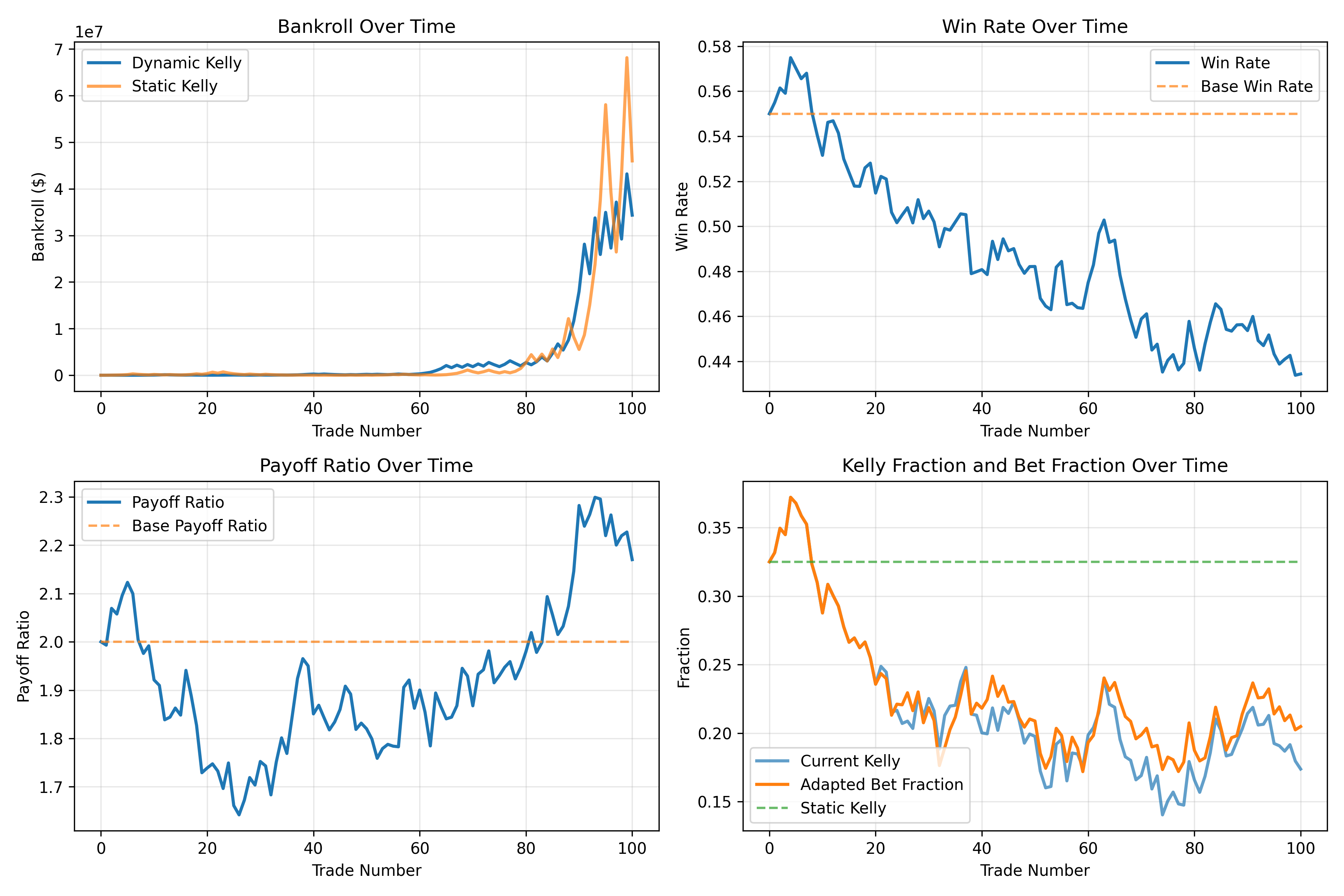
Real-World Example: Sports Betting with Streaks
Let’s consider a practical example of using Dynamic Bankroll Management for a sports bettor experiencing hot and cold streaks:
from keeks.bankroll import BankRoll
from keeks.binary_strategies.dynamic import DynamicBankrollManagement
import numpy as np
import matplotlib.pyplot as plt

# Create a bankroll with $5,000
bankroll = BankRoll(initial_funds=5000.0)

# Create a Dynamic Bankroll Management strategy
dbm = DynamicBankrollManagement(
    base_fraction=0.02,  # 2% base bet
    max_increase=0.5,    # Up to 50% increase (max 3% of bankroll)
    max_decrease=0.75,   # Up to 75% decrease (min 0.5% of bankroll)
    lookback_period=5    # Consider last 5 bets
)

# Let's simulate a betting season with streaks
# We'll create a sequence of 100 bets with some hot and cold streaks
np.random.seed(42)
results = []

# Start with normal 55% win rate
for i in range(30):
    results.append(1 if np.random.random() < 0.55 else -1)

# Cold streak (30% win rate for 20 bets)
for i in range(20):
    results.append(1 if np.random.random() < 0.3 else -1)

# Hot streak (70% win rate for 20 bets)
for i in range(20):
    results.append(1 if np.random.random() < 0.7 else -1)

# Back to normal 55% win rate
for i in range(30):
    results.append(1 if np.random.random() < 0.55 else -1)

# Track our bankroll and bet sizes
bankroll_history = [bankroll.current_funds]
bet_sizes = []
bet_fractions = []

# Simulate the bets
for i, result in enumerate(results):
    # Calculate the bet size
    current_streak = results[max(0, i-dbm.lookback_period):i]
    bet_fraction = dbm.calculate_bet_fraction(current_streak)
    bet_size = bet_fraction * bankroll.current_funds

    # Record the bet size
    bet_sizes.append(bet_size)
    bet_fractions.append(bet_fraction)

    # Apply the result
    if result == 1:
        # Win
        bankroll.update(bet_size)
    else:
        # Loss
        bankroll.update(-bet_size)

    # Record the new bankroll
    bankroll_history.append(bankroll.current_funds)

# Plot the results
fig, (ax1, ax2, ax3) = plt.subplots(3, 1, figsize=(12, 12), sharex=True)

# Plot the bankroll
ax1.plot(bankroll_history)
ax1.set_title('Bankroll Over Time')
ax1.set_ylabel('Bankroll ($)')
ax1.grid(True)

# Plot the bet sizes
ax2.plot(bet_sizes)
ax2.set_title('Bet Sizes Over Time')
ax2.set_ylabel('Bet Size ($)')
ax2.grid(True)

# Plot the bet fractions
ax3.plot(bet_fractions)
ax3.axhline(y=0.02, color='r', linestyle='--', label='Base Fraction (2%)')
ax3.set_title('Bet Fractions Over Time')
ax3.set_xlabel('Bet Number')
ax3.set_ylabel('Bet Fraction')
ax3.legend()
ax3.grid(True)

# Add vertical lines to indicate the streak changes
for ax in [ax1, ax2, ax3]:
    ax.axvline(x=30, color='g', linestyle='--', alpha=0.5, label='Start Cold Streak')
    ax.axvline(x=50, color='r', linestyle='--', alpha=0.5, label='Start Hot Streak')
    ax.axvline(x=70, color='b', linestyle='--', alpha=0.5, label='Return to Normal')

plt.tight_layout()
plt.show()

# Calculate final statistics
final_bankroll = bankroll_history[-1]
max_bankroll = max(bankroll_history)
min_bankroll = min(bankroll_history)
max_drawdown = (max_bankroll - min_bankroll) / max_bankroll * 100
total_return = (final_bankroll / 5000.0 - 1) * 100

print(f"Betting Statistics:")
print(f"  Initial bankroll: $5,000.00")
print(f"  Final bankroll: ${final_bankroll:.2f}")
print(f"  Total return: {total_return:.2f}%")
print(f"  Maximum bankroll: ${max_bankroll:.2f}")
print(f"  Minimum bankroll: ${min_bankroll:.2f}")
print(f"  Maximum drawdown: {max_drawdown:.2f}%")
print()
print(f"Bet Sizing Statistics:")
print(f"  Average bet size: ${np.mean(bet_sizes):.2f}")
print(f"  Maximum bet size: ${max(bet_sizes):.2f}")
print(f"  Minimum bet size: ${min(bet_sizes):.2f}")
print(f"  Average bet fraction: {np.mean(bet_fractions):.2%}")
When to Use Dynamic Bankroll Management
Dynamic Bankroll Management is particularly well-suited for:
- Streaky environments: Markets or sports with momentum or autocorrelation
- Varying edge scenarios: When your edge changes based on conditions
- Psychological alignment: When you want bet sizing to match your confidence
- Adaptive approach: When you prefer a system that responds to feedback
- Experienced bettors: Who can distinguish between variance and changing edge
Designing Your Dynamic Strategy
When implementing a Dynamic Bankroll Management strategy, consider these key parameters:
- Base strategy: Start with a solid foundation (Kelly, Fixed Fraction, etc.)
- Adjustment factors: How much to increase/decrease based on performance
- Lookback period: How many recent bets to consider when adjusting
- Limits: Maximum and minimum bet sizes to prevent extreme adjustments
- Triggers: What conditions trigger adjustments (wins/losses, volatility, etc.)
The optimal configuration depends on your betting style, the markets you’re in, and your risk tolerance.
Conclusion
Dynamic Bankroll Management represents a sophisticated approach to bet sizing that adapts to changing conditions. By adjusting your exposure based on recent performance and market conditions, it provides a flexible framework that can potentially outperform static strategies in certain environments.
While more complex to implement and tune than fixed strategies, DBM’s adaptability makes it particularly valuable in markets with streaks, changing edges, or varying volatility. For experienced bettors who can distinguish between normal variance and genuine shifts in their edge, DBM offers a powerful tool for optimizing bankroll growth while managing risk.
In our next post, we’ll explore the Naive Strategy, a simple approach that serves as a useful baseline for comparing more sophisticated bankroll management methods.
Stay in the loop
Get notified when I publish new posts. No spam, unsubscribe anytime.