Bankroll Management with Keeks: The Naive Strategy
In our previous posts, we’ve explored sophisticated bankroll management strategies from the Kelly Criterion to Dynamic Bankroll Management. Today, we’ll examine the Naive Strategy - a simple approach that serves as a useful baseline for comparison and, surprisingly, is still commonly used by many bettors and investors.
What is the Naive Strategy?
The Naive Strategy is exactly what it sounds like: betting the same fixed amount on every wager, regardless of your bankroll size, odds, or perceived edge. For example, you might decide to always bet $100 on each bet, no matter what.
This approach is sometimes called “flat betting” or “unit betting” and is one of the simplest bankroll management methods available. While it lacks the mathematical sophistication of other strategies, its simplicity makes it a popular choice for many casual bettors.
The Theory Behind the Naive Strategy
There’s not much theory behind the Naive Strategy - it’s more of a default approach than a calculated one. The formula is trivially simple:
Bet amount = Fixed amount
Unlike percentage-based strategies that scale with your bankroll, the Naive Strategy maintains the same absolute bet size regardless of your current funds.
Pros of the Naive Strategy
- Extreme simplicity: Requires no calculations or adjustments
- Psychological comfort: Easy to understand and implement
- Consistent exposure: Your absolute risk per bet remains constant
- No overreaction: Doesn’t increase bet sizes after winning streaks
- Beginner-friendly: Good starting point for novice bettors
Cons of the Naive Strategy
- No scaling: Doesn’t increase bet sizes as your bankroll grows
- Ruin risk: Can lead to bankruptcy if your bankroll gets too low
- Opportunity cost: Leaves money on the table during winning periods
- Ignores edge: Same bet size regardless of your advantage
- Not mathematically optimal: Significantly underperforms Kelly in the long run
Implementing the Naive Strategy with Keeks
Using the Naive Strategy with Keeks is straightforward:
from keeks.bankroll import BankRoll
from keeks.binary_strategies.naive import NaiveStrategy
from keeks.simulators.repeated_binary import RepeatedBinarySimulator
import matplotlib.pyplot as plt

# Create a bankroll with initial funds
initial_funds = 1000.0
bankroll = BankRoll(initial_funds=initial_funds)

# Create a Naive Strategy with $10 per bet
naive = NaiveStrategy(bet_amount=10.0)

# Simulate 1000 bets using the Naive Strategy
# Let's assume we have a 55% chance of winning with even money payouts
simulator = RepeatedBinarySimulator(
    payoff=1.0,
    loss=1.0,
    probability=0.55,
    trials=1000
)

# Run the simulation
simulator.evaluate_strategy(naive, bankroll)

# Plot the results
plt.figure(figsize=(10, 6))
plt.plot(bankroll.history)
plt.title('Bankroll Growth Using Naive Strategy ($10 per bet)')
plt.xlabel('Number of Bets')
plt.ylabel('Bankroll Size')
plt.grid(True)
plt.show()

# Print final results
final_bankroll = bankroll.history[-1]
growth_rate = (final_bankroll / initial_funds) ** (1 / 1000) - 1
print(f"Initial bankroll: ${initial_funds:.2f}")
print(f"Final bankroll: ${final_bankroll:.2f}")
print(f"Total return: {(final_bankroll/initial_funds - 1)*100:.2f}%")
print(f"Growth rate: {growth_rate:.2%} per bet")
Comparing Different Naive Strategies
Let’s compare how different fixed bet amounts perform on the same sequence of bets:
import numpy as np
from keeks.bankroll import BankRoll
from keeks.binary_strategies.naive import NaiveStrategy
from keeks.simulators.repeated_binary import RepeatedBinarySimulator
import matplotlib.pyplot as plt

# Set up our simulation parameters
win_probability = 0.55
payoff = 1.0
loss = 1.0
trials = 1000
initial_funds = 1000.0

# Create strategies with different fixed bet amounts
bet_amounts = [5.0, 10.0, 20.0, 50.0]
strategies = {}

for amount in bet_amounts:
    strategies[f"${amount:.0f} per bet"] = NaiveStrategy(bet_amount=amount)

# Create a simulator with fixed random seed for fair comparison
simulator = RepeatedBinarySimulator(
    payoff=payoff,
    loss=loss,
    probability=win_probability,
    trials=trials,
    random_seed=42  # Fixed seed ensures same sequence of wins/losses
)

# Run simulations
results = {}

for name, strategy in strategies.items():
    bankroll = BankRoll(initial_funds=initial_funds)
    simulator.evaluate_strategy(strategy, bankroll)
    results[name] = {
        "history": bankroll.history.copy(),
        "drawdowns": bankroll.drawdown_history.copy()
    }

# Plot the bankroll histories
plt.figure(figsize=(12, 8))
for name, data in results.items():
    plt.plot(data["history"], label=name)

plt.title('Comparison of Naive Strategies')
plt.xlabel('Number of Bets')
plt.ylabel('Bankroll Size')
plt.legend()
plt.grid(True)
plt.show()

# Calculate and display statistics
for name, data in results.items():
    history = data["history"]
    drawdowns = data["drawdowns"]

    final_value = history[-1]
    max_value = max(history)
    min_value = min(history)
    max_drawdown = max(drawdowns) * 100
    growth_rate = (final_value / initial_funds) ** (1 / trials) - 1

    print(f"{name}:")
    print(f"  Final bankroll: ${final_value:.2f}")
    print(f"  Growth rate: {growth_rate:.2%} per bet")
    print(f"  Maximum drawdown: {max_drawdown:.2f}%")
    print(f"  Minimum bankroll: ${min_value:.2f}")
    print()
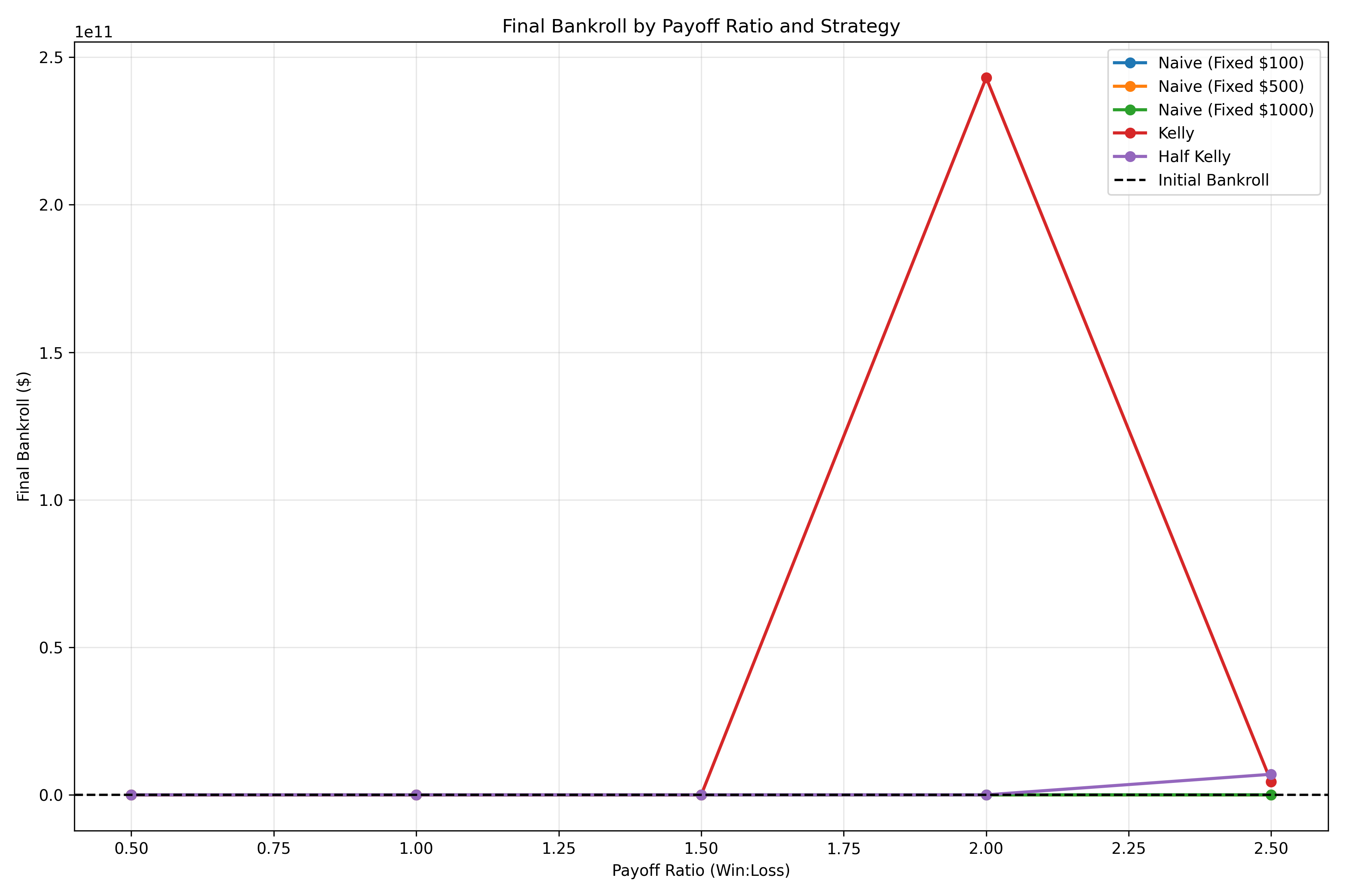
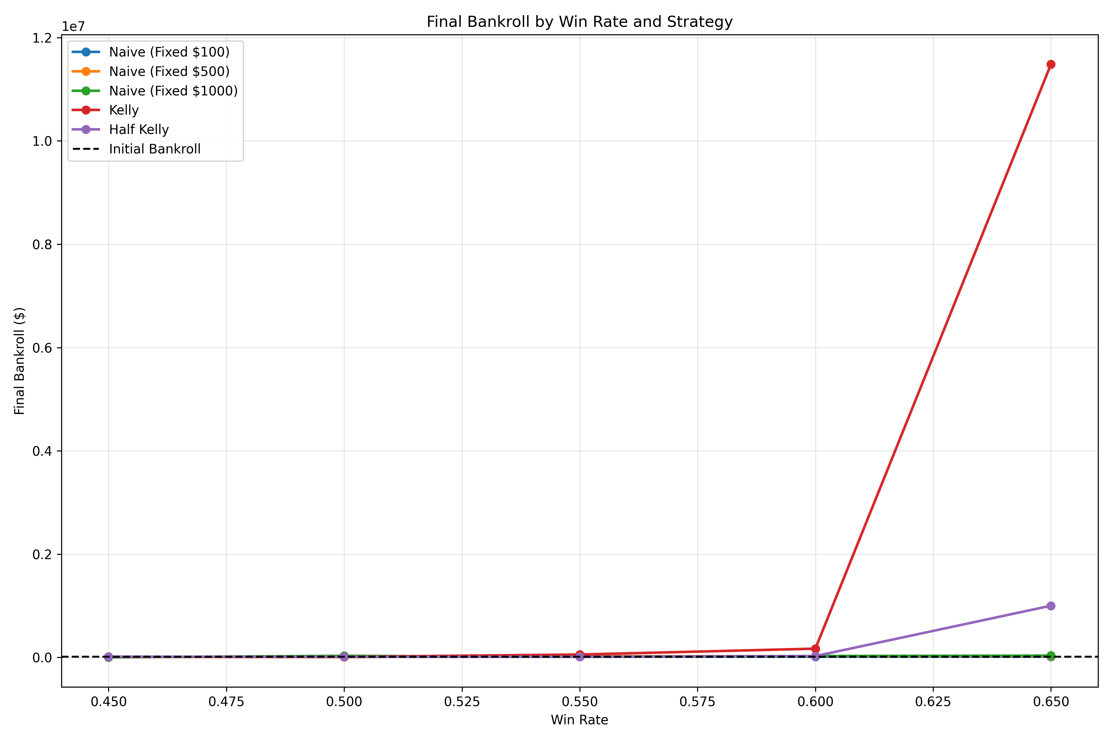
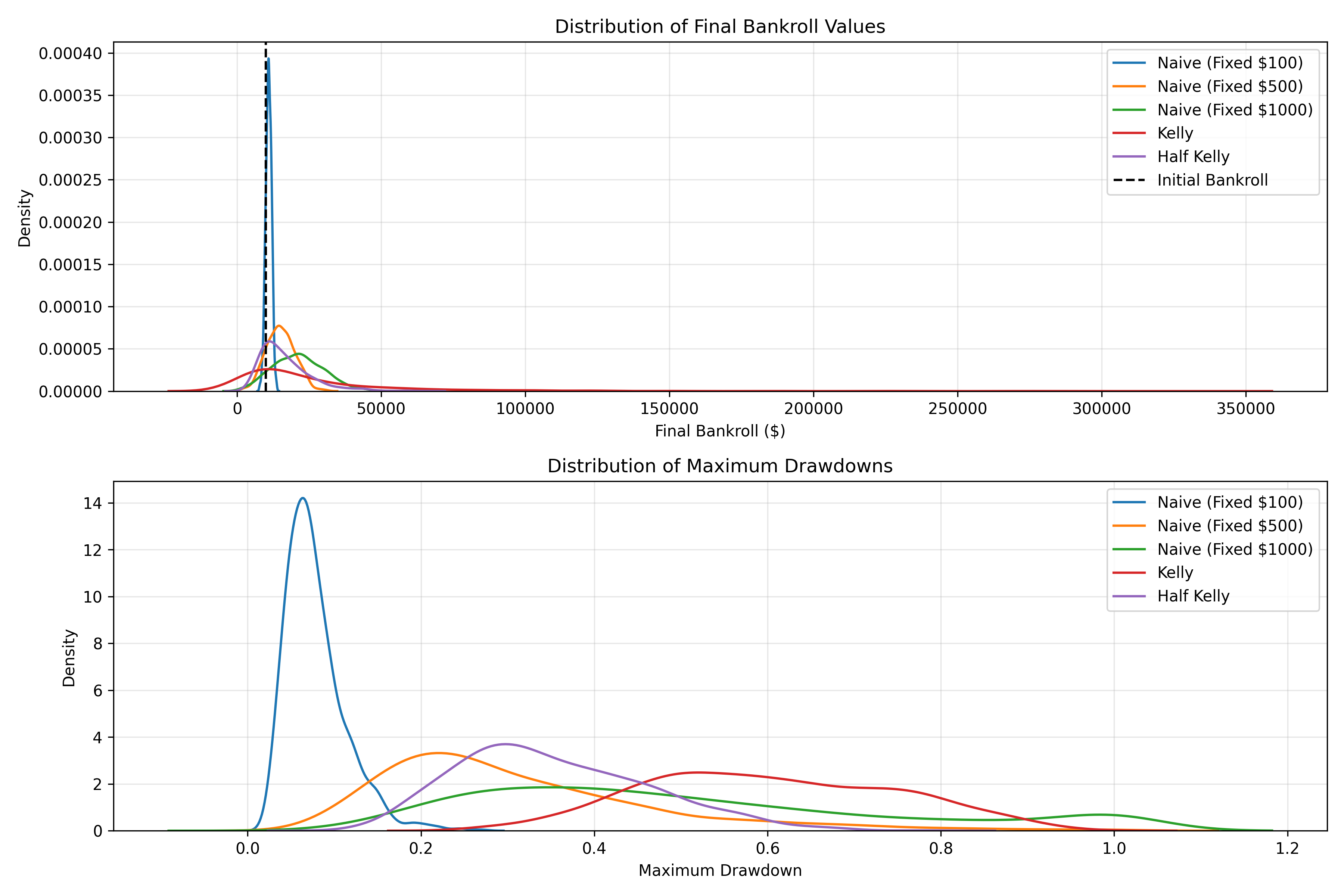
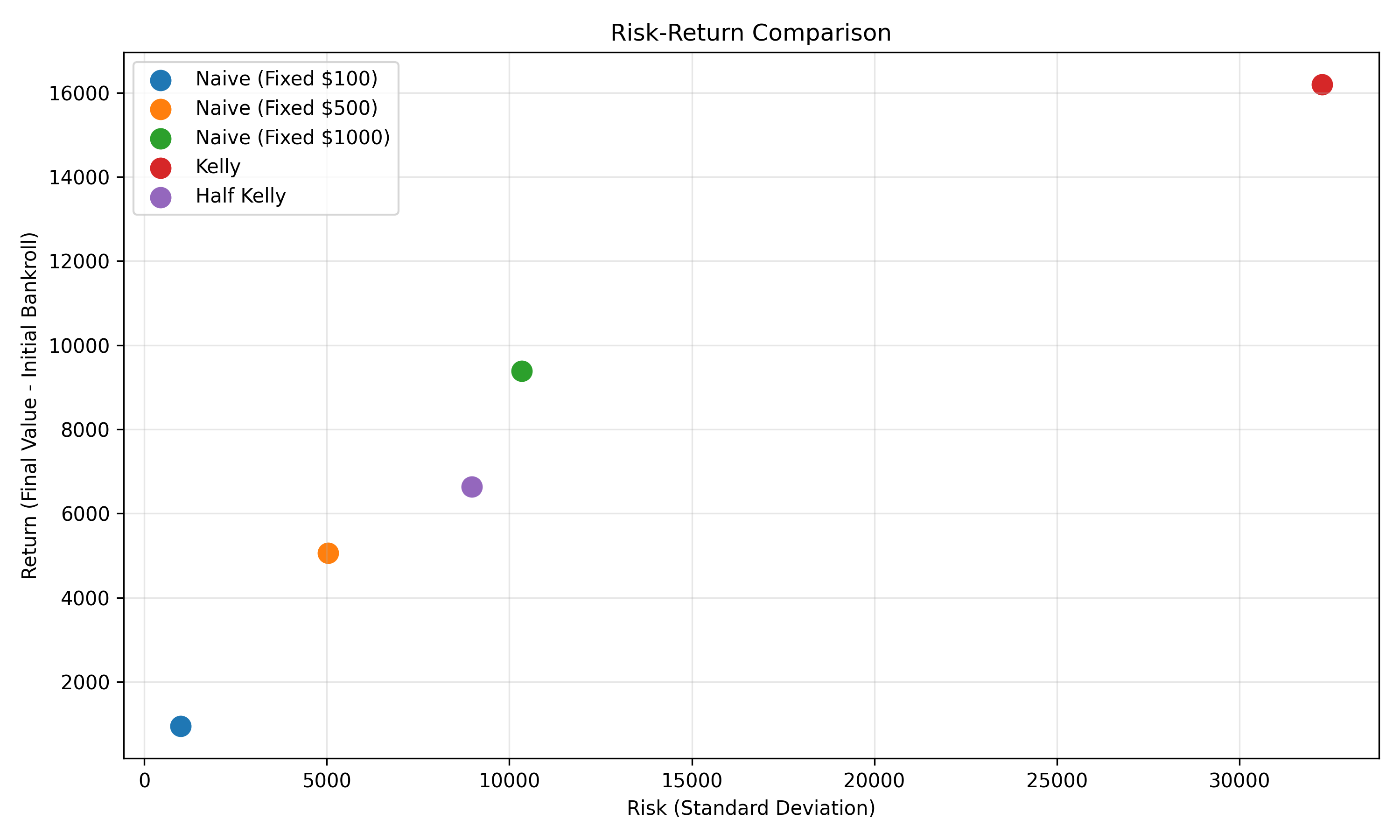
Comparing Naive Strategy with Other Strategies
Let’s see how the Naive Strategy compares to more sophisticated approaches:
from keeks.bankroll import BankRoll
from keeks.binary_strategies.kelly import KellyCriterion
from keeks.binary_strategies.fixed_fraction import FixedFraction
from keeks.binary_strategies.naive import NaiveStrategy
from keeks.simulators.repeated_binary import RepeatedBinarySimulator
import matplotlib.pyplot as plt

# Set up our simulation parameters
win_probability = 0.55
payoff = 1.0
loss = 1.0
trials = 1000
initial_funds = 1000.0

# Create strategies
kelly = KellyCriterion(payoff=payoff, loss=loss)
fixed_fraction = FixedFraction(fraction=0.03)
naive_10 = NaiveStrategy(bet_amount=10.0)
naive_30 = NaiveStrategy(bet_amount=30.0)

# Calculate the Kelly fraction for this scenario
kelly_fraction = kelly.calculate_bet_fraction(win_probability)
kelly_bet = kelly_fraction * initial_funds
print(f"Kelly fraction for this scenario: {kelly_fraction:.4f}")
print(f"Initial Kelly bet: ${kelly_bet:.2f}")

# Create a simulator with fixed random seed for fair comparison
simulator = RepeatedBinarySimulator(
    payoff=payoff,
    loss=loss,
    probability=win_probability,
    trials=trials,
    random_seed=42  # Fixed seed ensures same sequence of wins/losses
)

# Run simulations
results = {}
strategies = {
    "Kelly": kelly,
    "Fixed Fraction (3%)": fixed_fraction,
    "Naive ($10)": naive_10,
    "Naive ($30)": naive_30
}

for name, strategy in strategies.items():
    bankroll = BankRoll(initial_funds=initial_funds)
    simulator.evaluate_strategy(strategy, bankroll)
    results[name] = {
        "history": bankroll.history.copy(),
        "drawdowns": bankroll.drawdown_history.copy()
    }

# Plot the bankroll histories
plt.figure(figsize=(12, 8))
for name, data in results.items():
    plt.plot(data["history"], label=name)

plt.title('Naive vs Other Strategies')
plt.xlabel('Number of Bets')
plt.ylabel('Bankroll Size')
plt.legend()
plt.grid(True)
plt.show()

# Calculate and display statistics
for name, data in results.items():
    history = data["history"]
    drawdowns = data["drawdowns"]

    final_value = history[-1]
    max_drawdown = max(drawdowns) * 100
    growth_rate = (final_value / initial_funds) ** (1 / trials) - 1

    print(f"{name}:")
    print(f"  Final bankroll: ${final_value:.2f}")
    print(f"  Growth rate: {growth_rate:.2%} per bet")
    print(f"  Maximum drawdown: {max_drawdown:.2f}%")
    print()

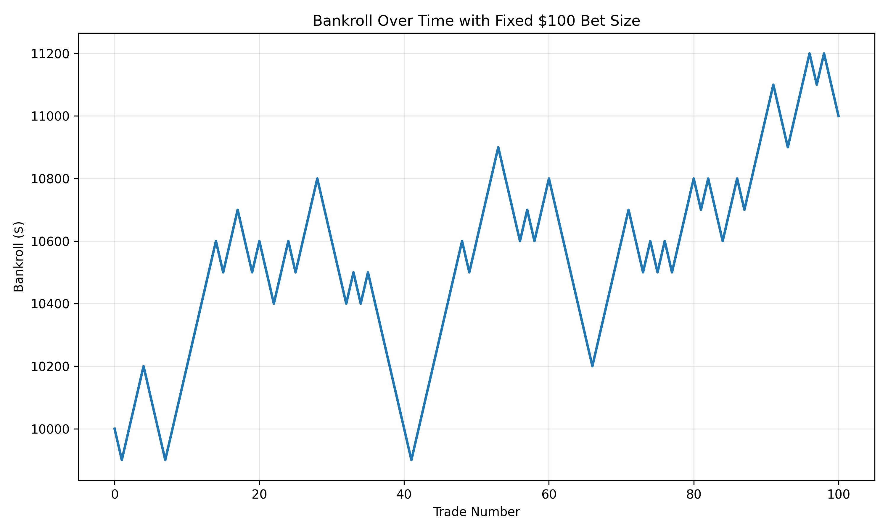
Real-World Example: Sports Betting with a Fixed Unit Size
Let’s consider a practical example of using the Naive Strategy for a sports bettor:
from keeks.bankroll import BankRoll
from keeks.binary_strategies.naive import NaiveStrategy
import numpy as np
import matplotlib.pyplot as plt

# Create a bankroll with $1,000
bankroll = BankRoll(initial_funds=1000.0)

# Create a Naive Strategy with $20 per bet
naive = NaiveStrategy(bet_amount=20.0)

# Let's simulate a betting season
# We'll create a sequence of 100 bets with varying win probabilities
np.random.seed(42)

# Define our betting scenario
num_bets = 100
win_probabilities = [0.53, 0.55, 0.58, 0.60]  # Different edges
payouts = [0.91, 0.91, 0.83, 0.77]  # Corresponding to -110, -110, -120, -130 odds

# Generate random bets with different edges
bets = []
for _ in range(num_bets):
    # Randomly select an edge/payout combination
    idx = np.random.randint(0, len(win_probabilities))
    prob = win_probabilities[idx]
    payout = payouts[idx]

    # Determine if the bet wins
    outcome = 1 if np.random.random() < prob else -1

    bets.append({
        "probability": prob,
        "payout": payout,
        "outcome": outcome
    })

# Track our bankroll and bet details
bankroll_history = [bankroll.current_funds]
bet_details = []

# Simulate the bets
for i, bet in enumerate(bets):
    # Calculate the bet amount (always the same with Naive Strategy)
    bet_amount = naive.bet_amount

    # Apply the result
    if bet["outcome"] == 1:
        # Win
        profit = bet_amount * bet["payout"]
        bankroll.update(profit)
        result = "Win"
    else:
        # Loss
        bankroll.update(-bet_amount)
        result = "Loss"

    # Record the bet details
    bet_details.append({
        "bet_number": i+1,
        "bet_amount": bet_amount,
        "probability": bet["probability"],
        "payout": bet["payout"],
        "result": result,
        "bankroll": bankroll.current_funds
    })

    # Record the new bankroll
    bankroll_history.append(bankroll.current_funds)

# Plot the results
plt.figure(figsize=(12, 6))
plt.plot(bankroll_history)
plt.title('Bankroll Using Naive Strategy ($20 per bet)')
plt.xlabel('Bet Number')
plt.ylabel('Bankroll ($)')
plt.grid(True)
plt.show()

# Calculate final statistics
final_bankroll = bankroll_history[-1]
max_bankroll = max(bankroll_history)
min_bankroll = min(bankroll_history)
max_drawdown = (max_bankroll - min_bankroll) / max_bankroll * 100
total_return = (final_bankroll / 1000.0 - 1) * 100

print(f"Betting Statistics:")
print(f"  Initial bankroll: $1,000.00")
print(f"  Final bankroll: ${final_bankroll:.2f}")
print(f"  Total return: {total_return:.2f}%")
print(f"  Maximum bankroll: ${max_bankroll:.2f}")
print(f"  Minimum bankroll: ${min_bankroll:.2f}")
print(f"  Maximum drawdown: {max_drawdown:.2f}%")

# Calculate win rate and ROI
wins = sum(1 for bet in bet_details if bet["result"] == "Win")
win_rate = wins / num_bets
roi = total_return / num_bets

print(f"\nPerformance Metrics:")
print(f"  Win rate: {win_rate:.2%}")
print(f"  ROI per bet: {roi:.2%}")
print(f"  Total bets: {num_bets}")

# What if we had used a percentage-based approach?
print(f"\nComparison with Fixed Fraction (2%):")
fixed_bankroll = 1000.0
fixed_history = [fixed_bankroll]

for i, bet in enumerate(bets):
    # Calculate the bet amount (2% of current bankroll)
    bet_amount = 0.02 * fixed_bankroll

    # Apply the result
    if bet["outcome"] == 1:
        # Win
        profit = bet_amount * bet["payout"]
        fixed_bankroll += profit
    else:
        # Loss
        fixed_bankroll -= bet_amount

    # Record the new bankroll
    fixed_history.append(fixed_bankroll)

# Calculate final statistics for Fixed Fraction
fixed_final = fixed_history[-1]
fixed_return = (fixed_final / 1000.0 - 1) * 100

print(f"  Naive final bankroll: ${final_bankroll:.2f}")
print(f"  Fixed Fraction final bankroll: ${fixed_final:.2f}")
print(f"  Naive return: {total_return:.2f}%")
print(f"  Fixed Fraction return: {fixed_return:.2f}%")
When to Use the Naive Strategy
The Naive Strategy is particularly well-suited for:
- Beginners: Who want to start with the simplest possible approach
- Small bankrolls: When percentage-based bets would be too small
- Recreational bettors: Who bet primarily for entertainment
- Short-term betting: For brief betting periods where bankroll growth is less important
- Testing systems: As a baseline for comparing more sophisticated strategies
Choosing Your Bet Size
When implementing a Naive Strategy, the key decision is your fixed bet amount. Here are some guidelines:
- Conservative approach: Bet 1-2% of your initial bankroll
- Moderate approach: Bet 3-5% of your initial bankroll
- Aggressive approach: Bet 5-10% of your initial bankroll
Remember that with the Naive Strategy, your bet size doesn’t adjust as your bankroll changes, so you need to choose an amount that:
- Won’t lead to ruin if you hit a losing streak
- Is large enough to make meaningful profits
- Aligns with your risk tolerance and betting goals
Conclusion
The Naive Strategy represents the simplest approach to bankroll management. While it lacks the mathematical sophistication and growth potential of strategies like Kelly or Fixed Fraction, its simplicity and consistency make it a popular choice for many bettors, especially beginners.
For those with positive expected value bets, the Naive Strategy will generally produce profits over time, though it will significantly underperform percentage-based strategies in the long run. Its main advantage is psychological - the fixed bet size is easy to understand and implement, and doesn’t lead to the potentially uncomfortable large bets that Kelly can recommend after winning streaks.
In our next and final post of this series, we’ll provide a comprehensive comparison of all the bankroll management strategies we’ve explored, helping you choose the right approach for your specific needs and preferences.
Stay in the loop
Get notified when I publish new posts. No spam, unsubscribe anytime.