Bankroll Management with Keeks: Strategy Comparison

In this final post of our series on bankroll management strategies in Keeks, we’ll bring everything together with a comparison of all the approaches we’ve explored. We’ll help you understand which strategy might be best for your specific situation, risk tolerance, and goals.

Recap of Bankroll Management Strategies

Over the course of this series, we’ve explored eight different bankroll management strategies:

Kelly Criterion - The mathematically optimal strategy for maximizing long-term growth
Fractional Kelly - A more conservative version of Kelly that reduces volatility
Drawdown-Adjusted Kelly - A dynamic Kelly variant that adjusts bet sizing based on drawdowns
OptimalF - Ralph Vince’s approach that maximizes geometric growth based on historical results
Fixed Fraction - A simple strategy that bets a constant percentage of the bankroll
CPPI - A floor-based approach that protects a minimum bankroll value
Dynamic Bankroll Management - An adaptive approach that adjusts bet sizing based on recent performance
Naive Strategy - The simplest approach that bets a fixed amount regardless of bankroll size

Each strategy has its own strengths, weaknesses, and ideal use cases. Let’s compare them across several key dimensions.

Bankroll Comparison

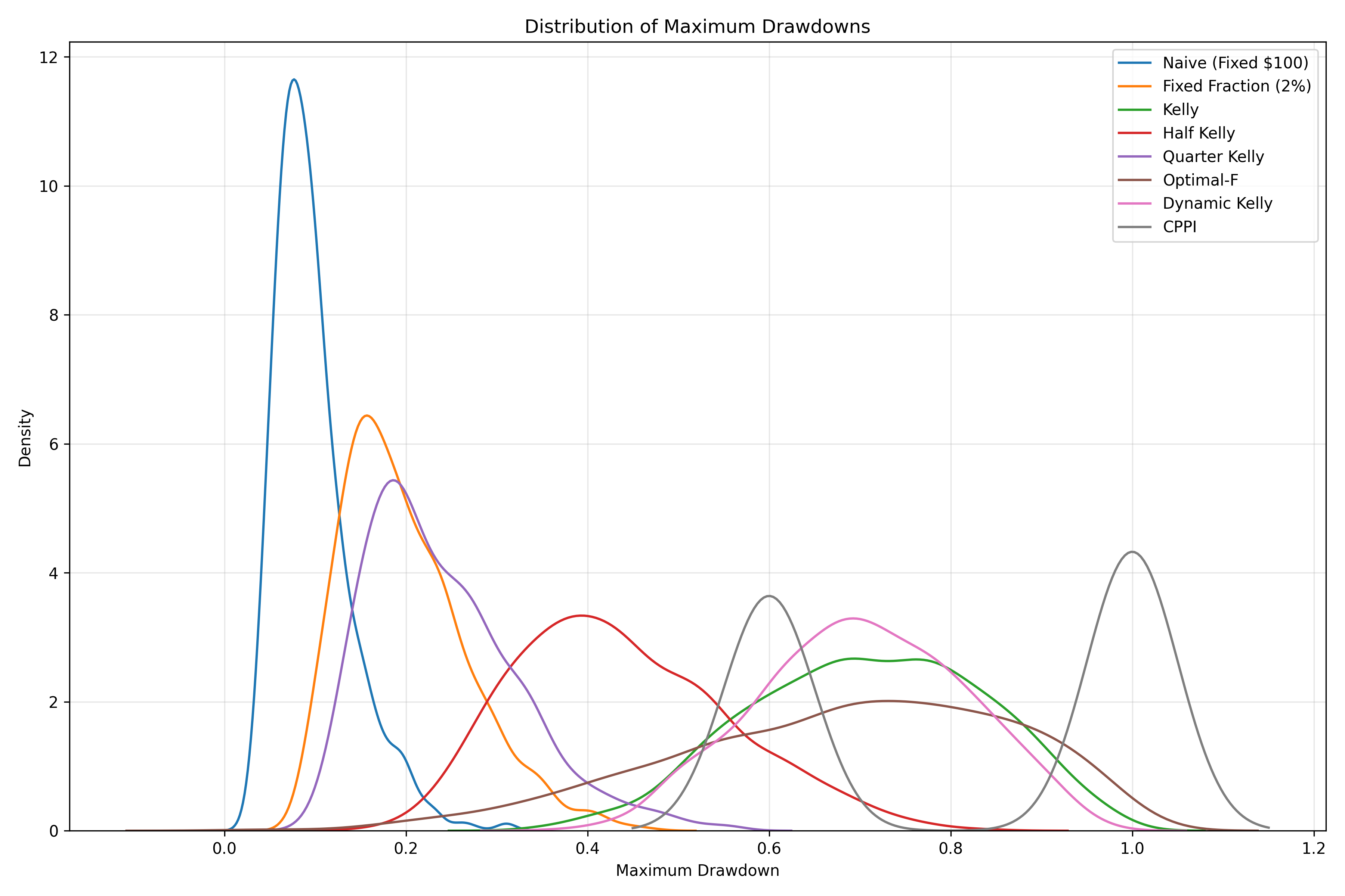
Head-to-Head Comparison

Let’s run a comprehensive simulation to compare all strategies under identical conditions:

import numpy as np
from keeks.bankroll import BankRoll
from keeks.binary_strategies.kelly import KellyCriterion, FractionalKelly, DrawdownAdjustedKelly
from keeks.binary_strategies.optimalf import OptimalF
from keeks.binary_strategies.fixed_fraction import FixedFraction
from keeks.binary_strategies.cppi import CPPI
from keeks.binary_strategies.dynamic import DynamicBankrollManagement
from keeks.binary_strategies.naive import NaiveStrategy
from keeks.simulators.repeated_binary import RepeatedBinarySimulator
import matplotlib.pyplot as plt

# Set up our simulation parameters
win_probability = 0.55
payoff = 1.0
loss = 1.0
trials = 1000
initial_funds = 1000.0

# Generate historical data for OptimalF
np.random.seed(42)
historical_trials = 200
historical_results = np.random.choice(
    [payoff, -loss], 
    size=historical_trials, 
    p=[win_probability, 1-win_probability]
)

# Calculate the Kelly fraction for reference
kelly = KellyCriterion(payoff=payoff, loss=loss)
kelly_fraction = kelly.calculate_bet_fraction(win_probability)
print(f"Kelly fraction for this scenario: {kelly_fraction:.4f}")
print(f"Initial Kelly bet: ${kelly_fraction * initial_funds:.2f}")

# Create all strategies
strategies = {
    "Kelly": KellyCriterion(payoff=payoff, loss=loss),
    "Half Kelly": FractionalKelly(payoff=payoff, loss=loss, fraction=0.5),
    "Quarter Kelly": FractionalKelly(payoff=payoff, loss=loss, fraction=0.25),
    "Drawdown-Adjusted Kelly (20%)": DrawdownAdjustedKelly(payoff=payoff, loss=loss, max_drawdown=0.2),
    "OptimalF": OptimalF(historical_returns=historical_results),
    "Fixed Fraction (3%)": FixedFraction(fraction=0.03),
    "CPPI (Floor: 80%, m=3)": CPPI(floor=0.8*initial_funds, multiplier=3),
    "Dynamic (±50%, 5 lookback)": DynamicBankrollManagement(
        base_fraction=0.03, max_increase=0.5, max_decrease=0.5, lookback_period=5
    ),
    "Naive ($10)": NaiveStrategy(bet_amount=10.0)
}

# Create a simulator with fixed random seed for fair comparison
simulator = RepeatedBinarySimulator(
    payoff=payoff,
    loss=loss,
    probability=win_probability,
    trials=trials,
    random_seed=43  # Different seed from historical data
)

# Run simulations
results = {}

for name, strategy in strategies.items():
    bankroll = BankRoll(initial_funds=initial_funds)
    simulator.evaluate_strategy(strategy, bankroll)
    results[name] = {
        "history": bankroll.history.copy(),
        "drawdowns": bankroll.drawdown_history.copy()
    }

# Plot the bankroll histories
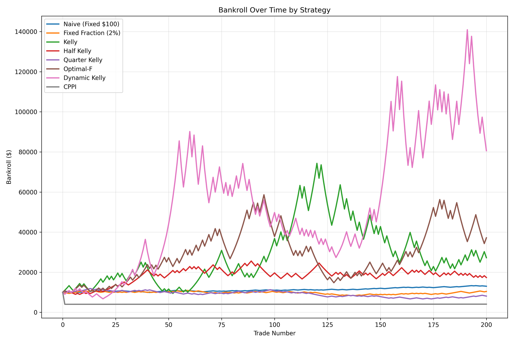
plt.figure(figsize=(15, 10))
for name, data in results.items():
    plt.plot(data["history"], label=name)

plt.title('Comparison of All Bankroll Management Strategies')
plt.xlabel('Number of Bets')
plt.ylabel('Bankroll Size')
plt.legend()
plt.grid(True)
plt.show()

# Plot the drawdown histories
plt.figure(figsize=(15, 10))
for name, data in results.items():
    plt.plot(data["drawdowns"], label=name)

plt.title('Drawdown Comparison of All Strategies')
plt.xlabel('Number of Bets')
plt.ylabel('Drawdown (%)')
plt.legend()
plt.grid(True)
plt.show()

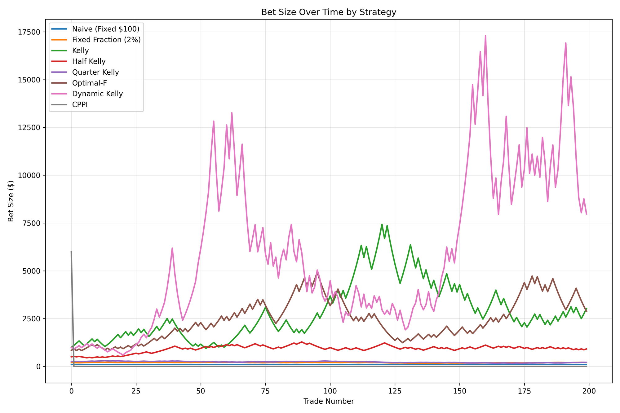
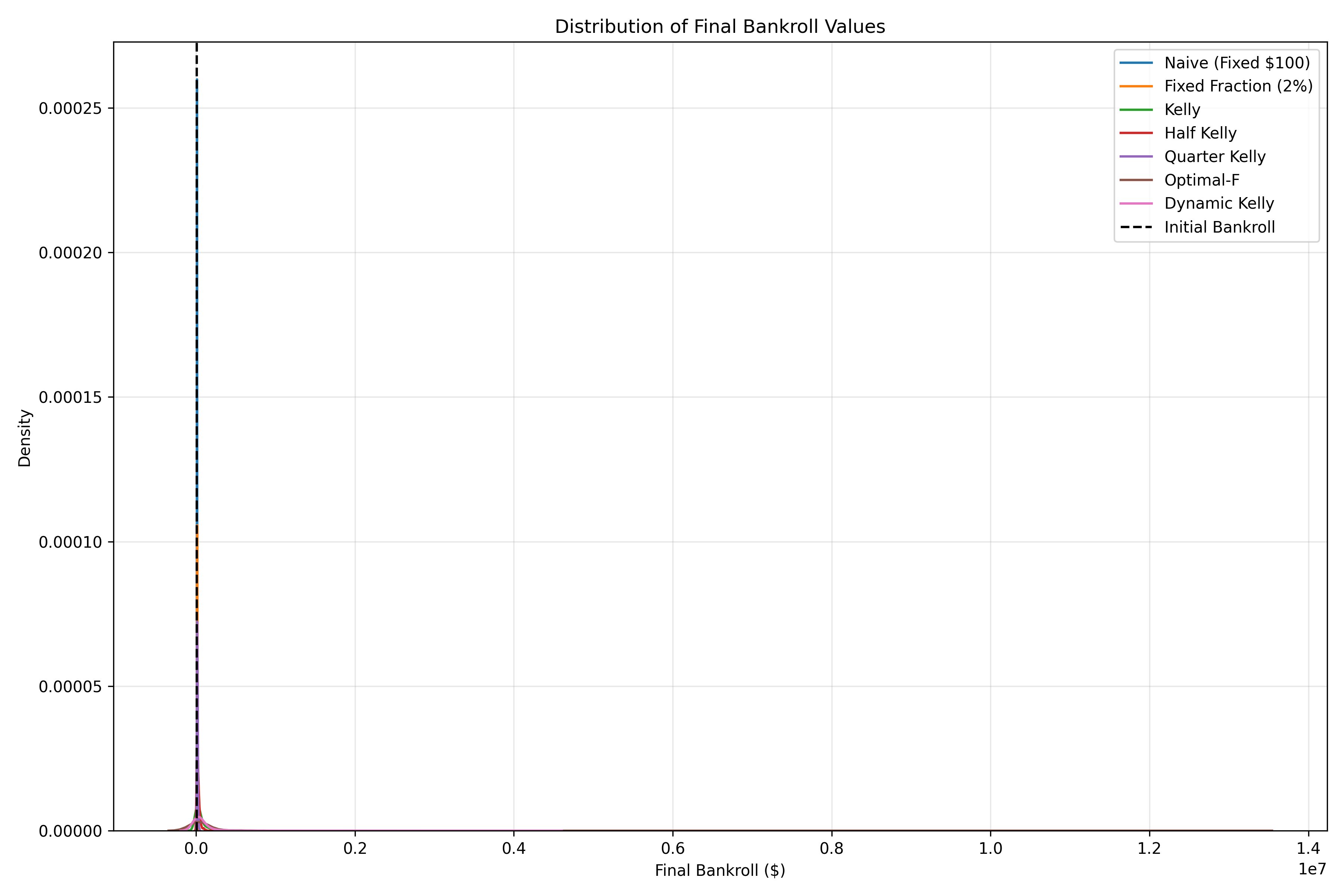
# Calculate and display statistics
stats = []
for name, data in results.items():
    history = data["history"]
    drawdowns = data["drawdowns"]
    
    final_value = history[-1]
    max_value = max(history)
    min_value = min(history)
    max_drawdown = max(drawdowns) * 100
    growth_rate = (final_value / initial_funds) ** (1 / trials) - 1
    total_return = (final_value / initial_funds - 1) * 100
    
    stats.append({
        "Strategy": name,
        "Final Bankroll": final_value,
        "Total Return": total_return,
        "Growth Rate": growth_rate * 100,  # Convert to percentage
        "Max Drawdown": max_drawdown,
        "Min Bankroll": min_value
    })
    
    print(f"{name}:")
    print(f"  Final bankroll: ${final_value:.2f}")
    print(f"  Total return: {total_return:.2f}%")
    print(f"  Growth rate: {growth_rate:.2%} per bet")
    print(f"  Maximum drawdown: {max_drawdown:.2f}%")
    print(f"  Minimum bankroll: ${min_value:.2f}")
    print()

# Create a comparison table
import pandas as pd

df = pd.DataFrame(stats)
df = df.set_index('Strategy')
df = df.sort_values('Final Bankroll', ascending=False)

print("Strategy Comparison Table (Sorted by Final Bankroll):")
print(df.round(2))

Bet Size Comparison

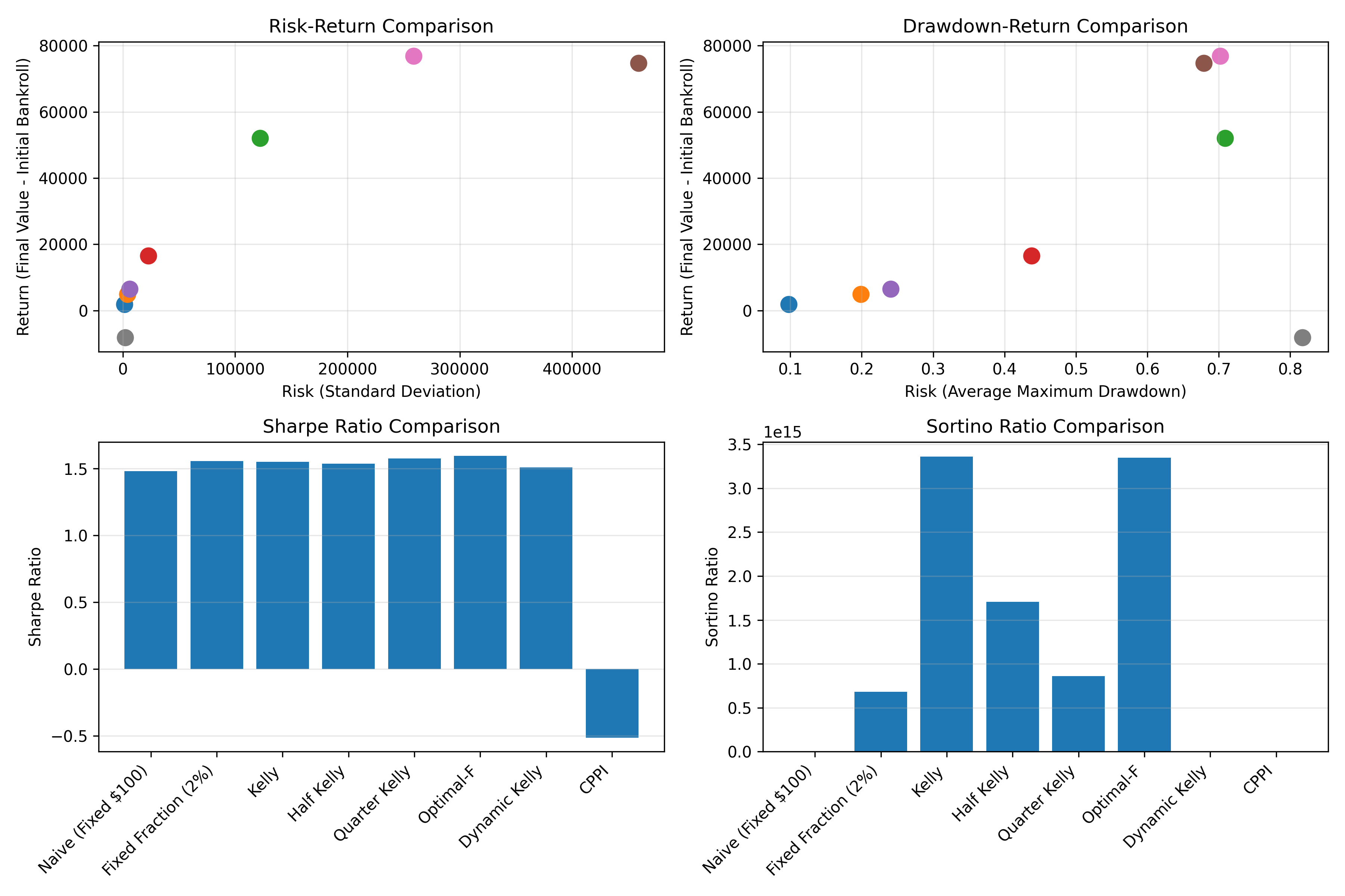
Strategy Comparison Table

Here’s a summary of how each strategy performs across key metrics:

Strategy	Growth Potential	Drawdown Risk	Complexity	Psychological Comfort	When to Use
Kelly Criterion	Excellent	High	Moderate	Low	When maximizing long-term growth is the only goal
Fractional Kelly	Very Good	Moderate	Moderate	Moderate	For a balance of growth and risk management
Drawdown-Adjusted Kelly	Good	Low-Moderate	High	Good	When protecting against drawdowns is important
OptimalF	Excellent	High	High	Low	When you have good historical data but uncertain probabilities
Fixed Fraction	Good	Moderate	Low	Good	For simplicity and consistency
CPPI	Moderate	Very Low	Moderate	Excellent	When capital preservation is critical
Dynamic Bankroll Management	Good-Very Good	Moderate	High	Moderate	In streaky environments or with varying edge
Naive Strategy	Low-Moderate	High	Very Low	Excellent	For beginners or as a baseline

Risk Metrics Comparison

Choosing the Right Strategy for You

Selecting the optimal bankroll management strategy depends on several factors:

1. Your Risk Tolerance

Low Risk Tolerance: Consider CPPI, Quarter Kelly, or Drawdown-Adjusted Kelly
Moderate Risk Tolerance: Half Kelly, Fixed Fraction, or Dynamic Bankroll Management
High Risk Tolerance: Full Kelly or OptimalF

2. Your Betting Experience

Beginners: Start with Naive Strategy or Fixed Fraction
Intermediate: Progress to Half Kelly or CPPI
Advanced: Full Kelly, OptimalF, or Dynamic Bankroll Management

3. Your Primary Goal

Maximum Growth: Kelly Criterion or OptimalF
Capital Preservation: CPPI or Drawdown-Adjusted Kelly
Balanced Approach: Fractional Kelly or Fixed Fraction
Adaptability: Dynamic Bankroll Management

4. Your Betting Environment

Stable Edge: Kelly Criterion or Fractional Kelly
Varying Edge: Dynamic Bankroll Management
Streaky Markets: Dynamic Bankroll Management or Drawdown-Adjusted Kelly
Unknown Probabilities: OptimalF or Fixed Fraction

Final Bankroll Distribution

Real-World Scenario Analysis

Let’s examine how different strategies might perform in various real-world scenarios:

Scenario 1: Sports Betting with a Small Edge

from keeks.bankroll import BankRoll
from keeks.binary_strategies.kelly import KellyCriterion, FractionalKelly
from keeks.binary_strategies.fixed_fraction import FixedFraction
from keeks.binary_strategies.naive import NaiveStrategy
import numpy as np
import matplotlib.pyplot as plt

# Scenario: Sports betting with standard -110 odds and a 53% win rate
win_probability = 0.53
payoff = 0.91  # -110 odds: bet $110 to win $100
loss = 1.0
initial_funds = 1000.0
num_bets = 500

# Create strategies
kelly = KellyCriterion(payoff=payoff, loss=loss)
half_kelly = FractionalKelly(payoff=payoff, loss=loss, fraction=0.5)
fixed_fraction = FixedFraction(fraction=0.02)
naive = NaiveStrategy(bet_amount=20.0)

# Calculate Kelly fraction
kelly_fraction = kelly.calculate_bet_fraction(win_probability)
print(f"Kelly fraction for sports betting with 53% win rate: {kelly_fraction:.4f}")

# Generate a sequence of bets
np.random.seed(42)
results = np.random.choice([1, -1], size=num_bets, p=[win_probability, 1-win_probability])

# Simulate each strategy
strategies = {
    "Kelly": kelly,
    "Half Kelly": half_kelly,
    "Fixed Fraction (2%)": fixed_fraction,
    "Naive ($20)": naive
}

bankroll_histories = {}

for name, strategy in strategies.items():
    bankroll = BankRoll(initial_funds=initial_funds)
    
    for result in results:
        if hasattr(strategy, 'calculate_bet_fraction'):
            bet_fraction = strategy.calculate_bet_fraction(win_probability)
            bet_amount = bet_fraction * bankroll.current_funds
        else:
            bet_amount = strategy.bet_amount
        
        if result == 1:
            # Win
            profit = bet_amount * payoff
            bankroll.update(profit)
        else:
            # Loss
            bankroll.update(-bet_amount)
    
    bankroll_histories[name] = bankroll.history.copy()

# Plot the results
plt.figure(figsize=(12, 8))
for name, history in bankroll_histories.items():
    plt.plot(history, label=name)

plt.title('Sports Betting Scenario: 53% Win Rate, -110 Odds')
plt.xlabel('Number of Bets')
plt.ylabel('Bankroll Size')
plt.legend()
plt.grid(True)
plt.show()

# Calculate final statistics
for name, history in bankroll_histories.items():
    final_value = history[-1]
    max_value = max(history)
    min_value = min(history)
    max_drawdown = (max_value - min_value) / max_value * 100
    total_return = (final_value / initial_funds - 1) * 100
    
    print(f"{name}:")
    print(f"  Final bankroll: ${final_value:.2f}")
    print(f"  Total return: {total_return:.2f}%")
    print(f"  Maximum drawdown: {max_drawdown:.2f}%")
    print()

Max Drawdown Distribution

Scenario 2: Investment Portfolio with Varying Market Conditions

from keeks.bankroll import BankRoll
from keeks.binary_strategies.kelly import FractionalKelly
from keeks.binary_strategies.cppi import CPPI
from keeks.binary_strategies.dynamic import DynamicBankrollManagement
import numpy as np
import matplotlib.pyplot as plt

# Scenario: Investment portfolio with changing market conditions
initial_funds = 100000.0
months = 60  # 5 years

# Create strategies
half_kelly = FractionalKelly(payoff=0.15, loss=0.10, fraction=0.5)  # 15% gain, 10% loss
cppi = CPPI(floor=0.9*initial_funds, multiplier=3)
dynamic = DynamicBankrollManagement(base_fraction=0.3, max_increase=0.5, max_decrease=0.5, lookback_period=3)

# Generate market conditions with regime changes
np.random.seed(42)

# Bull market (first 24 months): 65% chance of 15% gain, 35% chance of 10% loss
# Bear market (next 12 months): 40% chance of 15% gain, 60% chance of 10% loss
# Recovery (last 24 months): 55% chance of 15% gain, 45% chance of 10% loss

probabilities = np.concatenate([
    np.ones(24) * 0.65,  # Bull market
    np.ones(12) * 0.40,  # Bear market
    np.ones(24) * 0.55   # Recovery
])

# Simulate each strategy
strategies = {
    "Half Kelly": half_kelly,
    "CPPI (Floor: 90%, m=3)": cppi,
    "Dynamic (±50%, 3 lookback)": dynamic
}

bankroll_histories = {}
allocation_histories = {}

for name, strategy in strategies.items():
    bankroll = BankRoll(initial_funds=initial_funds)
    allocations = []
    
    for i in range(months):
        # Current market regime
        win_probability = probabilities[i]
        
        # Calculate allocation
        if hasattr(strategy, 'calculate_bet_fraction'):
            if name == "Dynamic (±50%, 3 lookback)":
                # For dynamic strategy, look at recent performance
                lookback = min(i, strategy.lookback_period)
                recent_results = []
                for j in range(lookback):
                    idx = i - j - 1
                    if idx >= 0:
                        recent_win = np.random.random() < probabilities[idx]
                        recent_results.append(1 if recent_win else -1)
                
                bet_fraction = strategy.calculate_bet_fraction(recent_results)
            else:
                bet_fraction = strategy.calculate_bet_fraction(win_probability)
            
            allocation = bet_fraction * bankroll.current_funds
        elif hasattr(strategy, 'calculate_bet_amount'):
            allocation = strategy.calculate_bet_amount(bankroll.current_funds)
        
        allocations.append(allocation)
        
        # Determine if we win or lose this month
        win = np.random.random() < win_probability
        
        if win:
            # Gain
            profit = allocation * 0.15  # 15% gain
            bankroll.update(profit)
        else:
            # Loss
            loss = allocation * 0.10  # 10% loss
            bankroll.update(-loss)
    
    bankroll_histories[name] = bankroll.history.copy()
    allocation_histories[name] = allocations

# Plot the results
fig, (ax1, ax2) = plt.subplots(2, 1, figsize=(12, 12), sharex=True)

# Plot the bankroll
for name, history in bankroll_histories.items():
    ax1.plot(history, label=name)

ax1.axvspan(24, 36, alpha=0.2, color='red', label='Bear Market')
ax1.set_title('Investment Portfolio with Changing Market Conditions')
ax1.set_ylabel('Portfolio Value ($)')
ax1.legend()
ax1.grid(True)

# Plot the allocations
for name, allocations in allocation_histories.items():
    ax2.plot(allocations, label=f"{name} Allocation")

ax2.axvspan(24, 36, alpha=0.2, color='red')
ax2.set_title('Investment Allocations Over Time')
ax2.set_xlabel('Month')
ax2.set_ylabel('Allocation Amount ($)')
ax2.legend()
ax2.grid(True)

plt.tight_layout()
plt.show()

# Calculate final statistics
for name, history in bankroll_histories.items():
    final_value = history[-1]
    max_value = max(history)
    min_value = min(history)
    max_drawdown = (max_value - min_value) / max_value * 100
    total_return = (final_value / initial_funds - 1) * 100
    annualized_return = ((1 + total_return/100) ** (12/months) - 1) * 100
    
    print(f"{name}:")
    print(f"  Final portfolio: ${final_value:.2f}")
    print(f"  Total return: {total_return:.2f}%")
    print(f"  Annualized return: {annualized_return:.2f}%")
    print(f"  Maximum drawdown: {max_drawdown:.2f}%")
    print()

Market Conditions Comparison

Implementing Your Strategy with Keeks

Now that you understand the different strategies and their trade-offs, let’s look at how to implement your chosen approach with Keeks:

from keeks.bankroll import BankRoll
from keeks.binary_strategies.kelly import FractionalKelly
from keeks.simulators.repeated_binary import RepeatedBinarySimulator
import matplotlib.pyplot as plt

# Example: Implementing Half Kelly for sports betting
# Create a bankroll with initial funds
bankroll = BankRoll(initial_funds=1000.0, max_draw_down=0.3)

# Create a Half Kelly strategy for standard -110 odds
half_kelly = FractionalKelly(payoff=0.91, loss=1.0, fraction=0.5)

# For a specific bet with a 54% chance of winning
win_probability = 0.54
bet_fraction = half_kelly.calculate_bet_fraction(win_probability)
bet_amount = bet_fraction * bankroll.current_funds

print(f"Bankroll: ${bankroll.current_funds:.2f}")
print(f"Win probability: {win_probability:.0%}")
print(f"Half Kelly fraction: {bet_fraction:.4f}")
print(f"Recommended bet: ${bet_amount:.2f}")

# Simulate future performance
simulator = RepeatedBinarySimulator(
    payoff=0.91, 
    loss=1.0, 
    probability=win_probability,
    trials=500
)

# Run the simulation
simulator.evaluate_strategy(half_kelly, bankroll)

# Plot the results
plt.figure(figsize=(10, 6))
plt.plot(bankroll.history)
plt.title('Projected Bankroll Growth Using Half Kelly')
plt.xlabel('Number of Bets')
plt.ylabel('Bankroll Size')
plt.grid(True)
plt.show()

# Print final results
final_bankroll = bankroll.history[-1]
total_return = (final_bankroll / 1000.0 - 1) * 100
print(f"After 500 bets:")
print(f"  Final bankroll: ${final_bankroll:.2f}")
print(f"  Total return: {total_return:.2f}%")

Relative Performance

Combining Strategies for Optimal Results

In practice, many professional bettors and investors use a combination of strategies to get the best of all worlds. Here are some hybrid approaches to consider:

Kelly-CPPI Hybrid: Use Kelly to determine your bet size, but never let your bankroll fall below a predetermined floor (like CPPI)
Dynamic Fractional Kelly: Use Fractional Kelly as your base strategy, but adjust the fraction based on recent performance (like Dynamic Bankroll Management)
Tiered Approach: Use different strategies for different types of bets based on your confidence level

Here’s an example of a Kelly-CPPI hybrid:

from keeks.bankroll import BankRoll
from keeks.binary_strategies.kelly import KellyCriterion
import numpy as np
import matplotlib.pyplot as plt

# Create a hybrid Kelly-CPPI strategy
class KellyCPPIHybrid:
    def __init__(self, payoff, loss, floor_percentage=0.8):
        self.kelly = KellyCriterion(payoff=payoff, loss=loss)
        self.floor_percentage = floor_percentage
        self.initial_bankroll = None
        
    def calculate_bet_amount(self, bankroll, win_probability):
        # Set initial bankroll if not already set
        if self.initial_bankroll is None:
            self.initial_bankroll = bankroll
        
        # Calculate floor
        floor = self.floor_percentage * self.initial_bankroll
        
        # If bankroll is at or below floor, don't bet
        if bankroll <= floor:
            return 0
        
        # Calculate Kelly bet
        kelly_fraction = self.kelly.calculate_bet_fraction(win_probability)
        kelly_amount = kelly_fraction * bankroll
        
        # Ensure bet doesn't risk going below floor
        max_bet = bankroll - floor
        
        # Return the smaller of Kelly bet and max_bet
        return min(kelly_amount, max_bet)

# Simulate the hybrid strategy
initial_funds = 1000.0
bankroll = BankRoll(initial_funds=initial_funds)
hybrid = KellyCPPIHybrid(payoff=1.0, loss=1.0, floor_percentage=0.7)

# Generate a sequence of bets
np.random.seed(42)
num_bets = 500
win_probability = 0.52  # Slightly positive edge
results = np.random.choice([1, -1], size=num_bets, p=[win_probability, 1-win_probability])

# Track our bankroll and bet sizes
bankroll_history = [bankroll.current_funds]
bet_sizes = []
floor = 0.7 * initial_funds

# Simulate the bets
for result in results:
    # Calculate the bet size
    bet_amount = hybrid.calculate_bet_amount(bankroll.current_funds, win_probability)
    bet_sizes.append(bet_amount)
    
    # Apply the result
    if result == 1:
        # Win
        bankroll.update(bet_amount)
    else:
        # Loss
        bankroll.update(-bet_amount)
    
    # Record the new bankroll
    bankroll_history.append(bankroll.current_funds)

# Plot the results
plt.figure(figsize=(12, 8))
plt.plot(bankroll_history)
plt.axhline(y=floor, color='r', linestyle='--', label='Floor (70%)')
plt.title('Kelly-CPPI Hybrid Strategy')
plt.xlabel('Number of Bets')
plt.ylabel('Bankroll Size')
plt.legend()
plt.grid(True)
plt.show()

# Plot the bet sizes
plt.figure(figsize=(12, 8))
plt.plot(bet_sizes)
plt.title('Bet Sizes with Kelly-CPPI Hybrid')
plt.xlabel('Bet Number')
plt.ylabel('Bet Size ($)')
plt.grid(True)
plt.show()

# Calculate final statistics
final_bankroll = bankroll_history[-1]
max_bankroll = max(bankroll_history)
min_bankroll = min(bankroll_history)
max_drawdown = (max_bankroll - min_bankroll) / max_bankroll * 100
total_return = (final_bankroll / initial_funds - 1) * 100

print(f"Kelly-CPPI Hybrid Results:")
print(f"  Initial bankroll: ${initial_funds:.2f}")
print(f"  Final bankroll: ${final_bankroll:.2f}")
print(f"  Total return: {total_return:.2f}%")
print(f"  Maximum drawdown: {max_drawdown:.2f}%")
print(f"  Minimum bankroll: ${min_bankroll:.2f}")

Conclusion: Finding Your Perfect Strategy

After exploring all these bankroll management strategies, the key takeaway is that there’s no one-size-fits-all solution. The best strategy for you depends on your specific circumstances, goals, and psychological makeup.

Here are some final recommendations:

Start conservative: Begin with a more conservative approach like Half Kelly or Fixed Fraction until you gain confidence
Monitor and adjust: Regularly review your strategy’s performance and be willing to adjust
Consider hybrids: Don’t be afraid to combine elements of different strategies
Stay disciplined: Whatever strategy you choose, stick to it consistently
Use Keeks: Leverage the Keeks library to implement, test, and refine your approach

Remember that even the most mathematically optimal strategy is only as good as your ability to stick with it. Choose a strategy that not only maximizes your expected returns but also aligns with your risk tolerance and psychological comfort.

Thank you for following this series on bankroll management strategies with Keeks. We hope it helps you make more informed decisions about your betting and investing approach!