Margin of Victory: Massey and Pythagorean
Most rating systems are told one bit per game: who won. elote v1.3.0 added two that get the whole scoreboard, and an optional score channel to carry it.
More information ought to mean better predictions, and it does. Feeding margins instead of outcomes is worth about a point of accuracy on college football, which is more than the gap between most of the systems in the library. What I did not expect was how much of the conventional wisdom around margin of victory fails when you actually measure it.
Two ways to read a scoreboard
Massey treats ratings as a least-squares fit to margins. Every game says r_winner - r_loser = margin, which is one equation, and a season is a big overdetermined system you solve:
M r = p
M = D - A, where D_ii is games played and A_ij is games between i and j; p_i is a competitor’s cumulative point differential. That matrix is a graph Laplacian, so its rows sum to zero and it is singular by construction. The standard repair is to replace the last row with all ones and the last entry of p with zero, pinning the ratings to zero mean.
The payoff is that Massey ratings are in points. The difference between two ratings is a predicted margin, which is a far more useful object than an abstract strength score.
Pythagorean expectation is older and much simpler. Bill James noticed that a baseball team’s win rate is predicted well by runs scored and runs allowed:
w = PF^k / (PF^k + PA^k)
Two properties make it the odd one out here. Its rating is already a win expectation, a number in [0, 1] that needs no logistic to be read as a probability. And it ignores the opponent graph completely: your rating depends only on your own points for and against, never on who supplied them.
Hold onto that second one.
Capping margin of victory does not help
Every serious computer ranking caps or discounts margin of victory. The BCS went further and banned it outright in 2002. So the obvious thing to test is where the cap should sit. I reshaped every margin in eight seasons of college football, preserving the loser’s score, and re-ran the week-by-week walk-forward:
| margin treatment | accuracy |
|---|---|
| cap at 3 | 0.7005 |
| cap at 7 | 0.7015 |
| cap at 14 | 0.7031 |
| cap at 21 | 0.7048 |
| cap at 28 | 0.7062 |
| cap at 35 | 0.7067 |
| raw margin | 0.7062 |
| sqrt(margin) | 0.7068 |
| win/loss only | 0.6965 |
There is no peak in the middle. Accuracy climbs monotonically as the cap loosens and flattens out once the cap stops binding on real games. Every cap tight enough to matter makes predictions worse, and the tightest one tested gives back more than half of what margins bought in the first place.
This is worth being clear about, because it is easy to read a cap as a modelling choice. It isn’t one. MOV caps exist so that a coach leading 49-0 has no incentive to keep throwing, and so a rating system cannot be gamed by running up the score. Those are good reasons. They are sportsmanship reasons. On this data the cap costs accuracy, and the BCS ban on margin was a policy decision that made the computer polls worse at their stated job.
The sqrt(margin) row is the other half of the story. Compressing a 49-point win to 7 and a 9-point win to 3 lands within noise of raw margins. Massey divides by the fitted rating spread before squashing to a probability, so a monotone rescaling of the margin units is largely absorbed. The system cares about the ordering of margins much more than their absolute size, which is exactly why clipping the ordering hurts and compressing it doesn’t.
Pythagorean’s one parameter cannot change a single prediction
Pythagorean has exactly one knob, the exponent k. It is fitted per sport: 2 for baseball, about 2.37 for football, around 14 for basketball. elote defaults to 2.37.
So I swept it, expecting a curve with an optimum:
| exponent k | accuracy |
|---|---|
| 1.00 | 0.6921 |
| 2.00 | 0.6921 |
| 2.37 | 0.6921 |
| 4.00 | 0.6921 |
| 10.00 | 0.6921 |
Identical to four decimal places across a tenfold range. That is not a flat optimum, it is a structural property of the model:
k     ratingA   ratingB   P(A beats B)
1.00   0.5992    0.5316      0.5684
2.37   0.7217    0.5745      0.6576
10.00  0.9824    0.7803      0.9401
The exponent moves the probability from 0.57 to 0.94 and never changes who is favoured. The reason is that PF^k / (PF^k + PA^k) is monotone in the ratio PF/PA for any positive k, and the log5 combination of two ratings exceeds 0.5 exactly when the first rating exceeds the second. So k cancels out of every binary decision the model makes.
Which means accuracy is structurally blind to the only parameter this model has. Log loss is not:
| exponent k | accuracy | log loss | Brier |
|---|---|---|---|
| 1.00 | 0.6921 | 0.5971 | 0.2051 |
| 1.50 | 0.6921 | 0.5795 | 0.1981 |
| 2.00 | 0.6921 | 0.5751 | 0.1962 |
| 2.37 | 0.6921 | 0.5783 | 0.1967 |
| 3.00 | 0.6921 | 0.5933 | 0.1997 |
| 6.00 | 0.6921 | 0.7548 | 0.2222 |
| 10.00 | 0.6921 | 1.0612 | 0.2449 |
There is the curve, and its minimum is at k = 2.0, not the 2.37 the library ships. The difference is small and 2.37 is a perfectly defensible default from the NFL literature, but college football is a different scoring environment with a much wider talent gap, and this data prefers James’ original baseball exponent.
The general lesson is worth more than the parameter. If your metric cannot see your parameter, you are measuring the wrong thing. Accuracy is a rank statistic: it only asks which side of 0.5 you landed on. Anything that changes confidence without changing order is invisible to it. If you are going to bet, or ensemble, or do anything at all with the probability rather than the pick, tune on log loss.
The opponent graph is the whole difference
Massey and Pythagorean read the same scoreboards and disagree constantly, because one of them knows who you played.
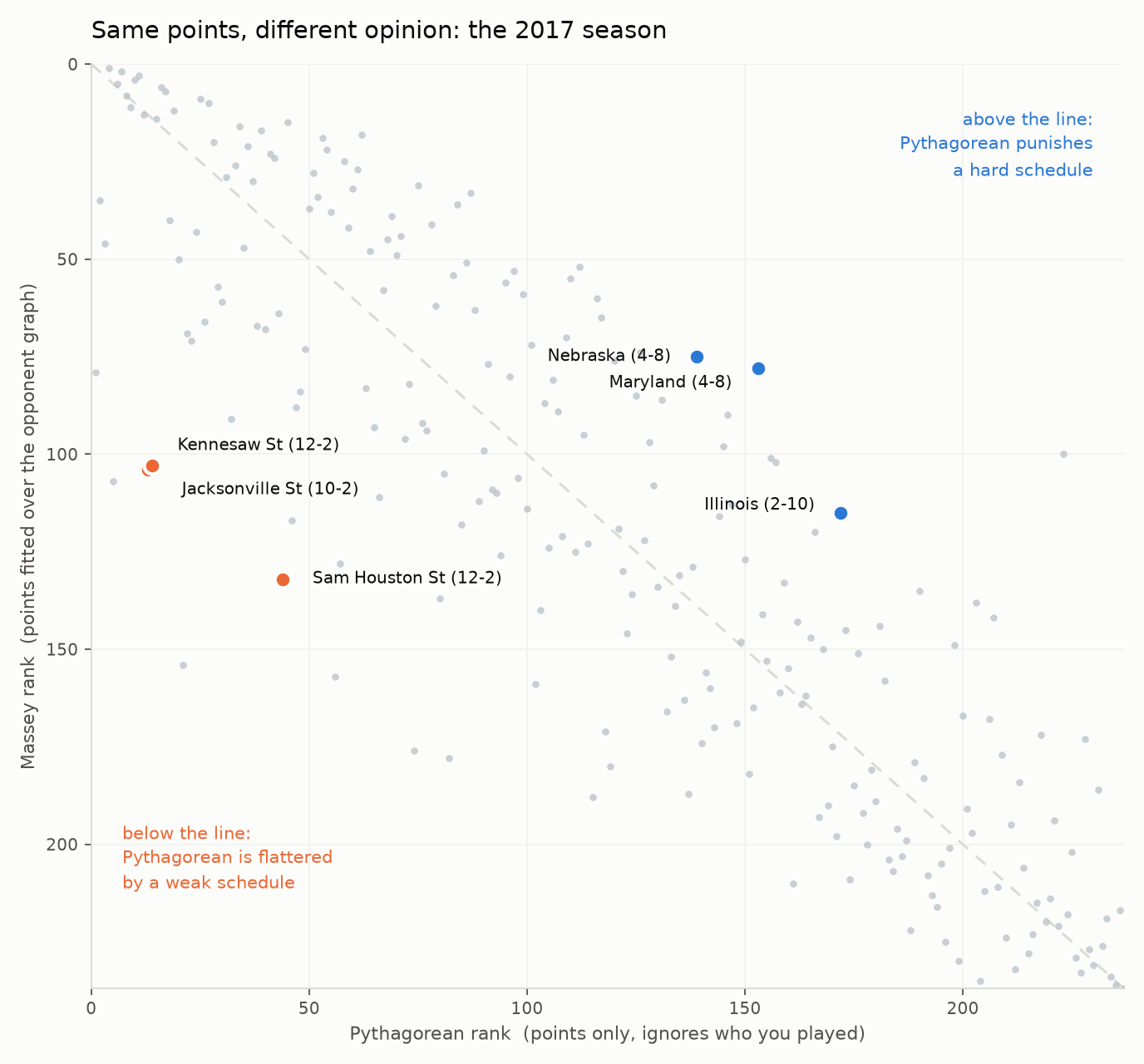
The extremes are exactly who you would nominate.
| team | record | point diff | Pythagorean | Massey |
|---|---|---|---|---|
| Kennesaw State | 12-2 | +204 | 13th | 104th |
| Jacksonville State | 10-2 | +166 | 14th | 103rd |
| Sam Houston State | 12-2 | +169 | 44th | 132nd |
| Illinois | 2-10 | -193 | 172nd | 115th |
| Nebraska | 4-8 | -128 | 139th | 75th |
| Maryland | 4-8 | -156 | 153rd | 78th |
Pythagorean has Kennesaw State, an FCS team, as the 13th best team in the country. They went 12-2 and outscored people by 204 points, and that is genuinely all Pythagorean knows. Massey has them 104th, because it can see that the wins came against teams that lost to everyone else.
The bottom half is the same effect inverted. Illinois went 2-10 and got outscored by 193 points, which reads as 172nd if you only look at the scoreboard. Massey has them 115th because it knows Illinois played Ohio State, Wisconsin and Penn State, and that being beaten by those teams says less about you than beating Southeast Missouri State does.
That is the entire 1.4 point accuracy gap between them in the walk-forward benchmark: 0.7062 for Massey, 0.6921 for Pythagorean. Same inputs, and the difference is one of them solving a system over the schedule and the other not.
What Massey needs in return
Fitting over the graph means Massey requires the graph to be connected. Its zero-mean pin is applied per connected component, so two competitors in separate components have ratings on unrelated scales, and comparing them produces a confident number with nothing behind it:
a.beat(b, scores=(20, 10))     # component 1
c.beat(d, scores=(30, 3))      # component 2
a.expected_score(c)            # 0.2910, and meaningless
I went looking for how often that bites in practice and the answer, on this data, is once. Of 6,385 predictions in the walk-forward, exactly one involved two teams with no path between them, because college football’s non-conference scheduling stitches the graph together almost immediately. Worth knowing before you point Massey at a sport with genuinely isolated leagues, and not worth worrying about here.
Pythagorean, of course, does not care at all. Having no graph means never having a disconnected one, and it will happily rate a competitor who has played a single game against an opponent nobody else has met. That is its weakness and its robustness, in the same sentence.
Picking between them
Massey when you have margins and a connected schedule, which is most league sports. It won the benchmark, its ratings are denominated in points, and the strength-of-schedule adjustment is doing real work rather than decorating the output.
Pythagorean when you want something that costs nothing. It is a constant-time update with no matrix, no graph and no refit, it reads out directly as a probability, and it lands within a point and a half of the best system in the library. For a first pass, or an ensemble member, or a sanity check on a fancier model, that is a good trade. Just don’t ask it who deserves the playoff spot.
And whichever you use, feed it the scores. That was worth more than the choice between them.
Reproducing
from elote import LambdaArena, MasseyCompetitor

arena = LambdaArena(lambda a, b, attributes=None: True, base_competitor=MasseyCompetitor)
arena.tournament([
    ("Alabama", "Auburn", None, None, 1.0, (31.0, 17.0)),   # scores as the last element
])
print(arena.expected_score("Alabama", "Auburn"))
pip install elote==1.3.1. The score channel is optional everywhere: leave it off and the same call rates on the result alone.
Stay in the loop
Get notified when I publish new posts. No spam, unsubscribe anytime.