Rocket Motor Optimization: Designing Thrust Profiles
Solid rocket motors are elegantly simple: a tube of propellant with a hole in the middle and a nozzle at one end. Light it, and the propellant burns from the inside surface outward. The shape of that internal cavity determines how the burn area changes over time, which determines the thrust profile.
Want constant thrust? Make the cavity a cylinder. Want high initial thrust that tapers off? Use a star-shaped cross-section. Want something more complex? You’ll need to optimize the geometry, and that’s where genetic algorithms earn their keep.
The Physics
When propellant burns, hot gases flow through the nozzle, producing thrust. The key relationships:
Burn rate depends on chamber pressure: $$r = a \cdot P_c^n$$
where a is a propellant-specific coefficient and n is the pressure exponent (typically 0.3-0.5).
Chamber pressure depends on burn surface area: $$P_c = \left(\frac{\rho \cdot a \cdot A_b \cdot c^*}{A_t}\right)^{\frac{1}{1-n}}$$
where ρ is propellant density, A_b is burn surface area, c* is characteristic velocity, and A_t is throat area.
Thrust is: $$F = P_c \cdot A_t \cdot C_F$$
where C_F is the thrust coefficient.
The burn surface area changes as the burn progresses. A cylindrical bore gets larger as it burns outward, so the area increases and thrust increases (progressive burn). A star pattern initially has large area (the star points), but the points burn away, reducing area and thrust (regressive in the later phase).
The Optimization Problem
Given a desired thrust profile (constant, boost-sustain, progressive), find the grain geometry that produces it.
The genome encodes a segmented star grain. The motor is split into six axial segments, each with its own bore radius and slot depth, plus four parameters shared across the whole grain. Sixteen genes in total, all normalized to [0, 1] and decoded into physical units:
def decode_genes(genes):
    bore_radii  = BORE_MIN  + genes[0:6]   * (BORE_MAX  - BORE_MIN)    # per segment
    slot_depths = SLOT_MIN  + genes[6:12]  * (SLOT_MAX  - SLOT_MIN)    # per segment
    n_slots     = NSLOTS_MIN + int(genes[12] * (NSLOTS_MAX - NSLOTS_MIN))
    slot_width  = WIDTH_MIN  + genes[13] * (WIDTH_MAX  - WIDTH_MIN)
    throat_d    = THROAT_D_MIN + genes[14] * (THROAT_D_MAX - THROAT_D_MIN)
    burn_rate_a = BURN_A_MIN + genes[15] * (BURN_A_MAX - BURN_A_MIN)
    ...
Per-segment control is what makes the interesting profiles reachable. A single bore radius for the whole grain can only produce the handful of curve shapes that one geometry gives you. Six segments that burn at different rates can be shaped against the target.
The fitness function runs a burn simulation and compares the resulting thrust curve to the target:
def thrust_curve_rms(genes, target_t, target_thrust):
    params = decode_genes(genes)

    # Simulate the burn with this geometry
    sim_t, sim_thrust = simulate_burn(**params)

    # Compare on the target's time grid
    sim_thrust_interp = np.interp(target_t, sim_t, sim_thrust)
    return float(np.sqrt(np.mean((sim_thrust_interp - target_thrust) ** 2)))
Note what this objective does not say anything about: how long the motor burns. Hold that thought.
The simulation is a time-stepping loop that updates geometry as propellant burns away:
while t < max_time and current_radius < R_outer:
    # Get current geometry
    perimeter, port_area = compute_star_geometry(
        current_radius, n_slots, current_depth, slot_width
    )

    # Chamber pressure from equilibrium
    A_b = perimeter * length
    k = rho * a * A_b * c_star / A_t
    P_c = k ** (1 / (1 - n))

    # Burn rate and thrust
    r = a * (P_c ** n)
    F = P_c * A_t * C_F

    # Update geometry
    current_radius += r * dt
    current_depth = max(0, current_depth - r * dt * 0.5)

    t += dt
Why GAs Work Here
This problem is perfect for genetic algorithms:
No analytical gradient: The thrust profile depends on a simulation. You can’t differentiate through a time-stepping loop with conditionals. Gradient-based methods don’t apply directly.
Mixed parameter types: bore radii, slot depths, slot width, throat diameter and burn rate coefficient are continuous. The number of star slots is discrete. GAs handle both naturally through the gene-to-parameter mapping, with no need to relax the integer or to run a separate search over it.
Multiple local optima: Different geometries can produce similar thrust profiles. The search space has many acceptable solutions, and the GA can find any of them.
Black-box simulation: The fitness function calls external physics code. The GA doesn’t need to know anything about the internals.
Target Profiles
Different missions need different thrust profiles:
Neutral (constant thrust): Good for sustained flight. The geometry must be designed so burn area stays approximately constant.
Boost-sustain: High initial thrust for liftoff, then lower thrust for efficient cruise. Requires more propellant to burn initially.
Progressive: Increasing thrust over time. Useful when payload gets lighter as fuel burns (though this applies more to liquid rockets).
Regressive: Decreasing thrust. Natural for many geometries and often acceptable.
The target curves are defined mathematically:
def create_target_thrust_curve(profile, duration, peak_thrust, dt):
    t = np.arange(0, duration, dt)

    if profile == "boost_sustain":
        thrust = np.where(t < 0.5, peak_thrust, peak_thrust * 0.4)
    elif profile == "progressive":
        thrust = peak_thrust * (t / duration) ** 0.5
    elif profile == "regressive":
        thrust = peak_thrust * (1 - 0.7 * t / duration)
    elif profile == "neutral":
        thrust = np.ones_like(t) * peak_thrust * 0.6

    return t, thrust
Running the Optimization
from parga import minimize

target_t, target_thrust = create_target_thrust_curve(
    profile="boost_sustain",
    duration=3.0,
    peak_thrust=5000,
)

def fitness(genes):
    return thrust_curve_rms(genes, target_t, target_thrust)

result = minimize(
    fitness,
    genome_length=16,
    bounds=(0.0, 1.0),
    population_size=100,
    generations=250,
    islands=4,
    seed=42,
    parallel=False,   # the burn sim is ~30ms, too fast to pay for process handoff
)
parallel=False is worth a note. The temptation with an expensive-looking objective is to
throw a process pool at it, but a single burn simulation takes about 30 milliseconds, and
handing a genome to another process and getting a float back costs more than that. ParGA’s
facade picks a strategy for you and reports which one it used; here it runs
rust_island, evaluating inside the Rust core across four islands.
Results
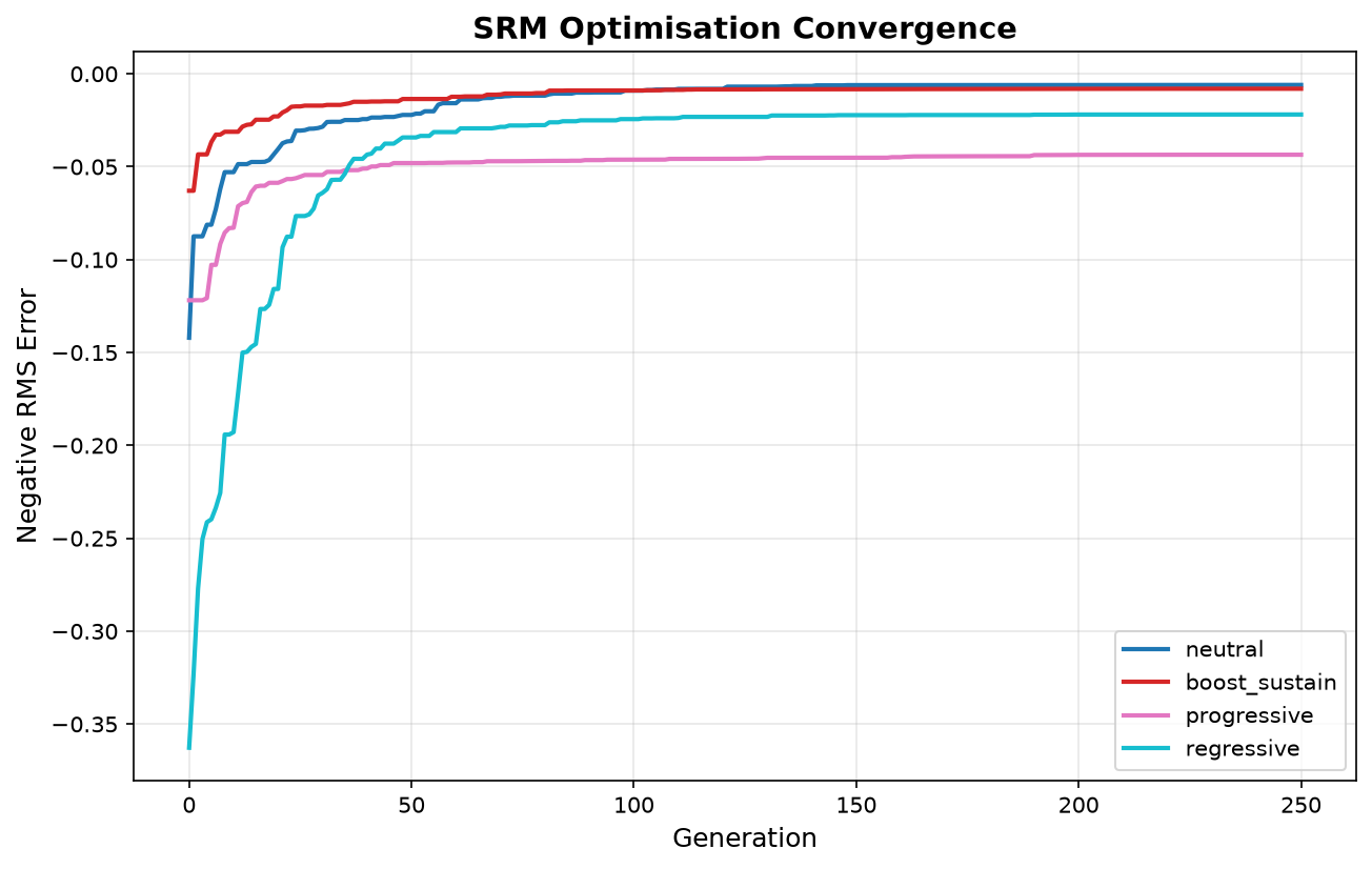
Four target profiles, 100 individuals, 250 generations, four islands, seed 42. Error is the RMS difference between the simulated and target thrust curves, as newtons and as a percentage of the mean target thrust:
| Profile | RMS error | as % of target | Time |
|---|---|---|---|
| neutral | 18 N | 0.6% | 63.3 s |
| boost-sustain | 21 N | 0.8% | 64.3 s |
| progressive | 129 N | 4.4% | 63.4 s |
| regressive | 47 N | 2.2% | 63.6 s |
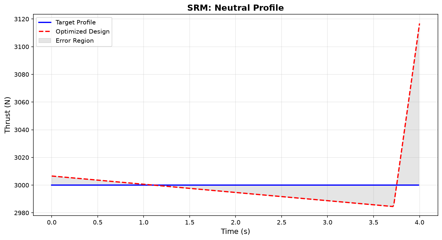
The ordering is the interesting part, and it is not the one I would have guessed.
Neutral is easiest. A flat thrust curve sounds like the hardest thing to hold, because burn area naturally changes as the grain regresses. But with six independently sized segments there are many ways to arrange an increasing bore against decreasing star points so the two cancel, and the optimizer finds one to within 0.6%.
Progressive is hardest, at 4.4%, roughly seven times the neutral error. Thrust has to climb through the whole burn, which means burn area must increase faster than the geometry naturally gives you, and that pushes against the bounds on every segment at once. The search runs out of geometry before it runs out of generations.
Regressive sits in the middle at 2.2%, which surprised me. Falling thrust is the natural behavior of a star grain, so I expected it to be the easy case. The catch is that the target also specifies a duration, and the geometries that fall off fastest do not burn for the requested time. In the regressive run the optimizer lands an excellent curve shape while overshooting burn duration by 2x, because the RMS objective weights curve shape and says nothing about total burn time.
That last one is a lesson about objectives, not about rockets. The optimizer answered the question I asked precisely. It was the wrong question, and nothing in the fitness value tells you that: 47 N of RMS error looks like a success right up until you read the burn time next to it.
Simulation Fidelity
The physics model here is simplified. Real solid rocket motor design involves:
- 3D grain geometry (not just 2D cross-section)
- Temperature-dependent burn rates
- Erosive burning at high gas velocities
- Structural integrity of the grain
- Combustion instabilities
- Nozzle erosion
Professional tools like openMotor or PROPEP handle these effects. The simplified model captures the essential relationship between geometry and thrust profile while being fast enough for optimization.
In a real design process, you’d use a cascade approach: optimize with the simplified model first, then verify and refine with higher-fidelity simulations.
Engineering Constraints
The optimization can include constraints beyond thrust matching:
Total impulse: The integral of thrust over time must meet mission requirements.
Burn time: Can’t be too short (structural loads) or too long (mission timeline).
Chamber pressure limits: Materials have maximum operating pressures.
Grain structural integrity: Thin sections can crack; long sections can deform.
These enter the fitness function as penalties:
if burn_time < min_time or burn_time > max_time:
    return -1e6

if max_pressure > pressure_limit:
    return -1e6
The Original Problem
The MATLAB code that became ParGA was written for a related problem: optimizing thrust vector control gains for a CubeSat attitude control system. Same concept (optimize parameters to match a desired profile), different physics.
That code evolved four populations independently, then merged them. The modern ParGA version uses continuous migration between islands, which finds better solutions more reliably on these simulation-based problems.
When Simulation-Based Optimization Shines
Rocket motors are a good example of a broader class of problems:
- You have a simulator (physics code, CAD software, FEA tool)
- You want to optimize design parameters
- Gradients aren’t available or are expensive to compute
- Multiple design objectives need balancing
Other examples: antenna design, structural optimization, aerodynamic shaping, material microstructure optimization. The GA treats the simulator as a black box and searches for good inputs.
Next: alloy composition optimization, where the fitness function involves materials science instead of rocket physics.
Stay in the loop
Get notified when I publish new posts. No spam, unsubscribe anytime.