Alloy Composition Optimization: Multi-Objective Materials Design
Designing a new alloy means balancing tradeoffs. You want high strength, but that often means high density. You want corrosion resistance, which requires expensive elements. You want low cost, but that limits your options.
Materials scientists spend careers navigating these tradeoffs, guided by physical intuition and hard-won experimental data. Computational tools can help explore the space of possibilities more systematically. This final case study shows how genetic algorithms optimize alloy compositions for multiple objectives.
The Materials Science Problem
An alloy is a mixture of elements. The proportions determine the properties. For a 5-component alloy, you have 4 independent composition variables (since fractions must sum to 1). Each composition gives a different set of properties: yield strength, hardness, density, corrosion resistance, melting point, cost.
Traditional alloy design focuses on one or two “base” elements with small additions of others. Stainless steel is mostly iron with chromium and nickel. Superalloys are mostly nickel with chromium, cobalt, aluminum, and titanium.
High-entropy alloys (HEAs) flip this convention: they contain five or more elements in roughly equal proportions. The high configurational entropy stabilizes unusual phases and produces exceptional properties. HEAs represent a vast, largely unexplored composition space.
Property Models
Real alloy properties come from experiments or quantum mechanical calculations (density functional theory). For optimization demos, we use simplified empirical models.
Rule of mixtures provides a baseline:
def rule_of_mixtures(fractions, element_values):
    return np.sum(fractions * element_values)
A 50% iron, 50% nickel alloy has approximately the average density of pure iron and pure nickel. This works reasonably for some properties and poorly for others.
Solid solution strengthening occurs when different-sized atoms distort the crystal lattice:
# Higher mixing entropy -> more lattice distortion -> higher strength
ss_factor = 1 + 0.5 * (mixing_entropy / 15)
The mixing entropy S_mix = -R * sum(x_i * ln(x_i)) measures how many ways atoms can arrange themselves. More components at equal fractions means higher entropy.
Synergy effects capture specific element interactions:
if {e1, e2} == {"Cr", "Ni"}:
    synergy *= 1.1  # Cr-Ni improves corrosion resistance
if {e1, e2} == {"Al", "Ti"}:
    synergy *= 1.15  # Al-Ti precipitates strengthen the alloy
These simplified models capture the flavor of real materials physics without requiring expensive computations.
Multi-Objective Fitness
Multiple properties need balancing. The fitness function combines them:
def multi_objective_fitness(fractions, elements, target_strength, target_hardness,
                            max_density, min_corrosion, weight_strength,
                            weight_hardness, weight_density, weight_corrosion):
    props = calculate_properties(fractions, elements)

    # Normalize relative to targets
    strength_score = min(props["yield_strength"] / target_strength, 1.5)
    hardness_score = min(props["hardness"] / target_hardness, 1.5)

    # Density: lower is better
    if props["density"] <= max_density:
        density_score = 1.0
    else:
        density_score = max_density / props["density"]

    # Corrosion: higher is better
    corrosion_score = min(props["corrosion_resistance"] / min_corrosion, 1.5)

    # Bonus for HEAs
    hea_bonus = 1.1 if props["is_hea"] else 1.0

    # Weighted combination
    fitness = (
        weight_strength * strength_score
        + weight_hardness * hardness_score
        + weight_density * density_score
        + weight_corrosion * corrosion_score
    ) * hea_bonus

    return fitness
The weights control priorities. For aerospace, density matters a lot. For tooling, hardness is paramount. For chemical processing, corrosion resistance dominates.
Genome Encoding
Each gene represents an element’s fraction:
elements = ["Fe", "Ni", "Cr", "Co", "Mn"]
n_elements = len(elements)

def fitness(genes):
    # Normalize to sum to 1
    fractions = genes / (np.sum(genes) + 1e-10)
    return -multi_objective_fitness(fractions, elements, ...)
The GA optimizes the relative proportions. Normalization ensures valid compositions (fractions summing to 1).
Bounds prevent any element from going to zero:
result = minimize(
    fitness,
    genome_length=n_elements,
    bounds=(0.01, 1.0),  # Minimum 1% for each element
    ...
)
This constraint reflects practical manufacturing: trace amounts are hard to control precisely.
Example Alloy Systems
The benchmark optimizes several alloy families:
Stainless Steel (Fe-Cr-Ni-Mn): The workhorse of corrosion-resistant alloys. Chromium forms a protective oxide layer. Nickel stabilizes the austenite phase. Manganese is a cheap austenite stabilizer.
Ni-based Superalloy (Ni-Cr-Co-Al-Ti): High-temperature strength for jet engines. Aluminum and titanium form strengthening precipitates. Chromium and cobalt provide oxidation resistance.
Cantor HEA (Fe-Ni-Cr-Co-Mn): The most famous high-entropy alloy, discovered by Brian Cantor. Equal parts of five transition metals, exceptional strength and ductility.
Lightweight High-Strength (Al-Ti-V-Cr-Fe): Emphasizes low density while maintaining strength. Aluminum and titanium provide the lightweight base; chromium and vanadium add strength.
Results
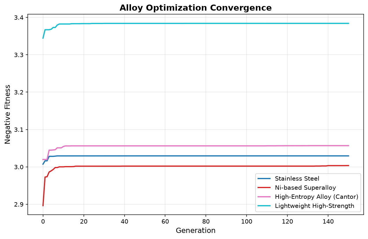
Four alloy systems, each optimized against its own targets. Every run finishes in about 0.22 seconds, which is worth pausing on: the property model is pure NumPy over five elements, so ParGA’s facade picks the plain Rust strategy and never reaches for a process pool it would only lose time to.
| System | Elements | Strength | Hardness | Density | HEA |
|---|---|---|---|---|---|
| Stainless Steel | Fe-Cr-Ni-Mn | 382 MPa | 247 HV | 7.45 | No |
| Ni-based Superalloy | Ni-Cr-Co-Al-Ti | 415 MPa | 276 HV | 6.66 | Yes |
| High-Entropy Alloy (Cantor) | Fe-Ni-Cr-Co-Mn | 389 MPa | 262 HV | 7.88 | Yes |
| Lightweight High-Strength | Al-Ti-V-Cr-Fe | 445 MPa | 307 HV | 5.70 | Yes |
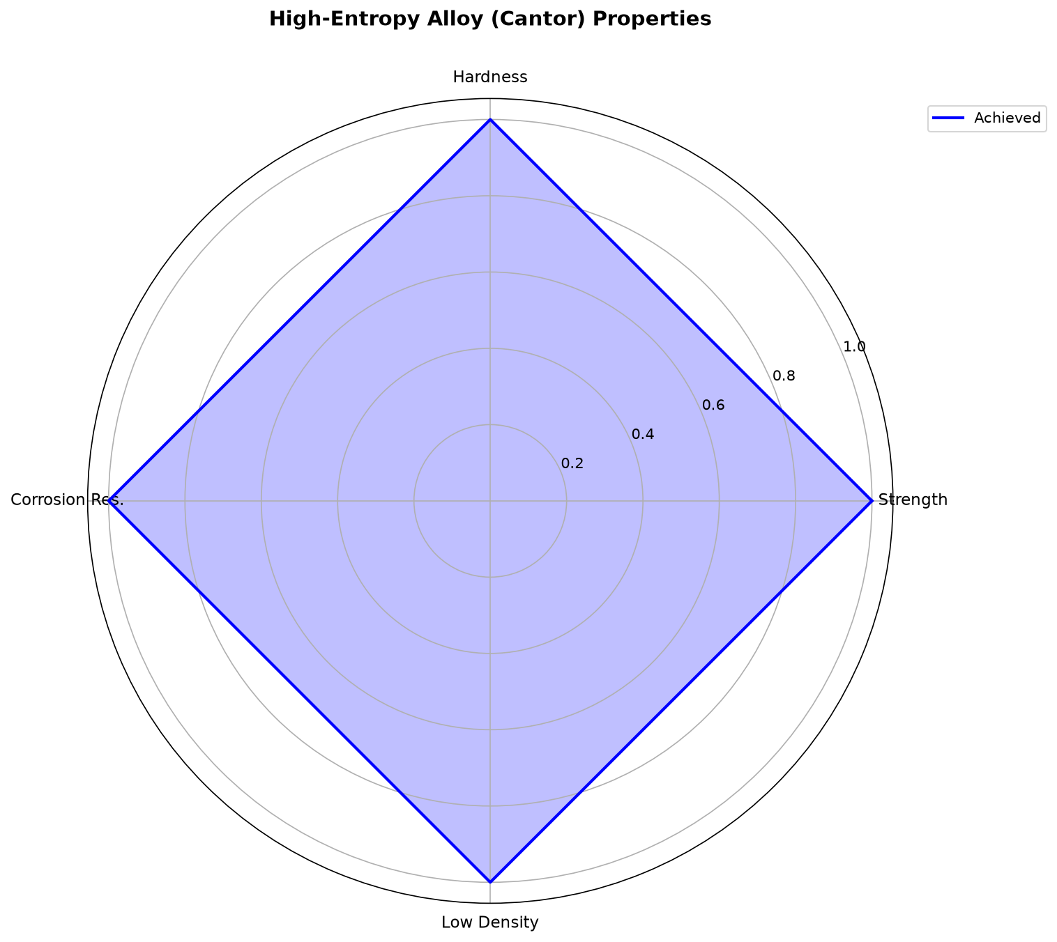
The Cantor result is the interesting one. The mixing entropy term rewards even mixing, so equiatomic is the intuitive answer, and it is not what the optimizer picks:
Fe: 7.0% Ni: 11.7% Cr: 47.8% Co: 19.8% Mn: 13.8%
Chromium takes nearly half the alloy. Entropy is only one term in the objective, and chromium is carrying corrosion resistance and strength at once, so the optimizer spends mixing entropy to buy those and stops as soon as it has enough. Which brings up the more interesting thing the run exposed.
The optimizer will sit exactly on your cliff edge
The “high-entropy alloy” flag isn’t decorative. It gates a strength bonus, which makes it a step change in the fitness landscape. Look at what every system’s mixing entropy converged to:
Stainless Steel              11.50 J/mol/K
Ni-based Superalloy          11.50 J/mol/K
High-Entropy Alloy (Cantor)  11.50 J/mol/K
Lightweight High-Strength    11.50 J/mol/K
Four different element sets, four different property targets, and one entropy value to four
significant figures. The threshold in the code was s_mix > 11.5, and the optimizer found
the cheapest composition that clears it and spent nothing more. Every joule of mixing entropy
above the line is wasted budget that could have gone to strength or density, so it went there
instead.
That is correct behavior against a discontinuous objective, and it is the sort of thing you only notice if your report prints the quantity next to the flag it drives. A bonus with a hard threshold does not encourage the property, it pins solutions to the boundary.
Where you put that threshold is therefore a real modelling decision, not a formality.
Miracle and Senkov define a high-entropy alloy as one with a mixing entropy of at least
1.5R, which is 12.47 J/mol/K. That number is worth deriving rather than rounding, because
an equiatomic four-element alloy tops out at R ln 4 = 11.53 and so can never qualify,
while a five-element one reaches R ln 5 = 13.38 and comfortably can. Set the cutoff a
little below 11.53 and every well-mixed quaternary passes; set it at 1.5R and the stainless
steel system correctly reports No while the three five-component systems still qualify.
Soft constraints are not constraints
One more result worth reading carefully. The lightweight system asks for a maximum density of 5.5 g/cm³ and the optimizer returns 5.70. The constraint is a ratio penalty:
if props["density"] <= max_density:
    density_score = 1.0
else:
    density_score = max_density / props["density"]
Exceeding by 3.6% costs 3.5% of one weighted term. The strength gained by spending that density is worth more, so the optimizer takes the trade, correctly, and reports a number that violates the stated limit without flagging it as a violation.
If a limit is real, it needs to be a rejection or a penalty steep enough to never be worth paying, and the report needs to say when it was breached. A ratio penalty expresses a preference, not a constraint.
Compared to Real Materials Discovery
This demo captures the workflow but not the complexity:
In reality: Properties come from expensive experiments or quantum calculations taking hours to days per composition. Machine learning surrogates trained on existing data can speed evaluation.
In reality: Phase stability matters. Not every composition forms a single-phase solid solution. Multi-phase microstructures have different properties than the constituent phases.
In reality: Processing affects properties. The same composition with different heat treatments gives different strength. The optimization must include processing parameters.
In reality: Uncertainty matters. Property measurements have error bars. Robust optimization accounts for this.
The genetic algorithm approach scales to these realistic scenarios. Swap in a machine learning model trained on DFT data. Add phase diagram constraints. Include processing parameters in the genome. The GA doesn’t care where the fitness number comes from.
Multi-Objective Considerations
The weighted-sum approach has limitations. It finds a single “best” solution according to the weights. Different weights give different solutions.
True multi-objective optimization finds the Pareto frontier: all compositions where you can’t improve one property without worsening another. NSGA-II and similar algorithms do this natively.
For ParGA’s current single-objective framework, you can approximate Pareto exploration by running multiple optimizations with different weight combinations, or by using the island model with different objectives on different islands (a form of implicit multi-objective search).
Connection to the Series
This case study closes the loop on ParGA’s development journey:
The original MATLAB code evolved populations to optimize thrust vector gains. The Rust rewrite generalized the approach. The island model improved solution quality. The case studies demonstrate real applications.
Molecular clusters, protein folding, rocket motors, alloy design: different physics, same algorithmic skeleton. Define a fitness function that measures how good a solution is. Let evolution explore the space. Trust the population dynamics to balance exploration and exploitation.
What’s Next for ParGA
The library is functional but not finished. Potential improvements:
Multi-objective optimization: Native Pareto frontier tracking, NSGA-II or MOEA/D algorithms.
Adaptive parameters: Mutation and crossover rates that change during evolution based on population diversity.
Better parallelism: GPU acceleration for fitness evaluation, distributed island models across machines.
More genome types: Permutation genomes for sequencing problems, integer genomes for discrete variables.
Hybrid algorithms: Combine GAs with local search (memetic algorithms) for faster convergence on smooth landscapes.
The architecture supports these extensions. The core loop stays the same.
Summary
Eight posts, one story: taking a useful MATLAB script and turning it into a modern, performant, well-documented library. AI code agents did the heavy lifting of translation and boilerplate. Rust provides performance and safety. PyO3 makes it accessible to Python users. Island models improve solution quality.
Genetic algorithms aren’t magic. They’re a reasonable default when you don’t have gradients, when the landscape is rugged, when you can afford many fitness evaluations. The case studies here show that “reasonable default” covers a surprising range of real problems.
ParGA is open source. Try it on your optimization problems. File issues when it breaks. Contribute improvements when you find them.
Stay in the loop
Get notified when I publish new posts. No spam, unsubscribe anytime.