Nine Bankroll Strategies Under Four Kinds of Stress
keeks v0.6.0 ships a benchmark. Nine staking strategies, ten scenarios, 200 paths each, 500 bets per path, and a CSV plus charts committed in the repo so the numbers are checkable rather than claimed.
I’ve written about Kelly with real payoffs as an individual piece of math. This is the whole staking library run head to head, and the interesting result is not which strategy grows fastest. It’s which ones survive being wrong.
The setup
The base scenario is a bettor with a genuine 55% edge at even money, no transaction cost, and a perfectly known probability. From there, four axes make life harder: the edge shrinks or grows, transaction costs appear, the probability estimate gets noisy, and the per-bet size cap tightens.
Two design decisions make the numbers mean something.
Common random numbers. Outcomes are drawn once per path from a seeded generator and replayed by trial index, so trial 400 of a given path resolves the same way for all nine strategies. Seeding the global RNG would not be enough, because the simulator only draws when a bet is actually placed, and a strategy that skips a trial would shift every later outcome and get a different world to play in.
Fresh state per run. Every scenario, strategy, path combination builds a new bankroll and a new strategy instance, because simulators mutate the bankroll in place and CPPI and Dynamic carry state between calls.
The result is reproducible in the strict sense. I ran it against keeks==0.6.0 in a clean virtualenv and diffed my CSV against the one committed in the repo: byte for byte identical.
The base case: growth costs drawdown
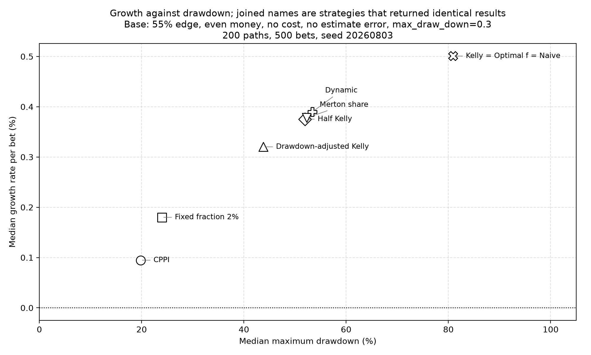
| Strategy | First bet | Median terminal | 5th pct | Median max drawdown |
|---|---|---|---|---|
| Kelly | 10.0% | 12,234 | 493 | 81% |
| Optimal f | 10.0% | 12,234 | 493 | 81% |
| Naive | 10.0% | 12,234 | 493 | 81% |
| Dynamic | 5.0% | 7,019 | 1,288 | 53% |
| Merton share | 5.1% | 6,612 | 1,312 | 52% |
| Half Kelly | 5.0% | 6,529 | 1,316 | 52% |
| Drawdown-adjusted Kelly | 4.0% | 4,957 | 1,377 | 44% |
| Fixed fraction 2% | 2.0% | 2,460 | 1,297 | 24% |
| CPPI | 4.0% | 1,605 | 866 | 20% |
Starting from 1,000. Full Kelly turns it into a median 12,234 and does so while spending part of nearly every path down 81% from its own high-water mark. Half Kelly gives up 47% of the terminal wealth to cut the drawdown from 81% to 52%. That is the textbook trade and it is nice to see it fall out of a simulation rather than an argument.
The 5th percentile column is the one I’d actually look at. Full Kelly’s worst 5% of paths end at 493, below where they started, after 500 bets with a real 55% edge. Half Kelly’s end at 1,316.
Three strategies returning identical numbers
Kelly, Optimal f and Naive produce bit-identical results here, which is a genuine algebraic identity rather than a coincidence of this scenario. Naive sizes at expected value per unit of payoff, (p*a - q*l) / a, which is p - q*l/a. This library’s Kelly, which accounts for a loss multiplier, is p/l - q/a. Set l = 1 and both collapse to p - q/a.
So whenever you lose your entire stake, betting the expected value per unit of payoff is Kelly. They only come apart when the loss multiplier isn’t 1:
payoff=1.0 loss=1.0  -> kelly 0.1000  naive 0.1000
payoff=1.0 loss=0.5  -> kelly 0.6500  naive 0.3250
payoff=2.0 loss=0.5  -> kelly 0.8750  naive 0.4375
At half loss, Kelly bets twice what Naive does. The benchmark’s base scenario is even money, so the three coincide, and the chart labels them as one point rather than pretending three markers are hiding under each other.
The axis that actually matters
Cost barely moves anything: at a 5% transaction cost, Kelly’s median terminal drops from 12,234 to 6,475 and no strategy stops early. Edge changes the numbers in the direction you’d expect.
Estimate error is a different animal. This axis perturbs the probability handed to the strategy while the simulator settles against the true one, which is exactly the real situation: your model says 55% and the world is running at 55%, but your model’s individual numbers are noisy.
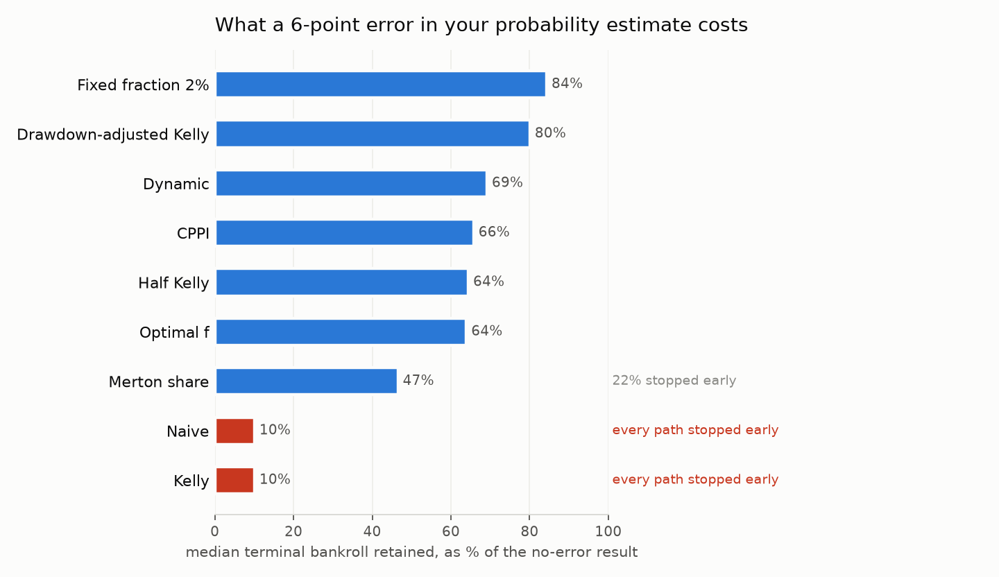
With 6 points of standard deviation on the estimate:
| Strategy | Base | Noise 0.03 | Noise 0.06 | Early stops at 0.06 |
|---|---|---|---|---|
| Optimal f | 12,234 | 12,174 | 7,826 | 0% |
| Dynamic | 7,019 | 6,340 | 4,857 | 0% |
| Half Kelly | 6,529 | 5,397 | 4,208 | 0% |
| Drawdown-adjusted Kelly | 4,957 | 4,397 | 3,971 | 0% |
| Merton share | 6,612 | 5,474 | 3,079 | 23% |
| Fixed fraction 2% | 2,460 | 2,420 | 2,076 | 0% |
| Kelly | 12,234 | 5,096 | 1,238 | 100% |
| Naive | 12,234 | 5,096 | 1,238 | 100% |
| CPPI | 1,605 | 1,240 | 1,056 | 0% |
Full Kelly loses 90% of its terminal wealth and every single path stops early. Not some. All 200. The edge is still there, the bettor still has it, and the strategy still destroys itself, because Kelly sizes off the number you hand it and a number that is sometimes 0.61 gets a bet sized for 0.61.
Optimal f loses least in absolute terms and keeps a growth rate of 0.0041 against Kelly’s 0.0004. That is v0.5.0’s change earning its keep: Optimal f now sizes off its historical or expected win rate while keeping the per-trial probability only as a gate. It doesn’t believe any individual estimate, so no individual estimate can hurt it.
Two ways of reading the same table, and both are worth stating. In relative terms the flat strategies look best, because Fixed fraction 2% keeps 84% of a small number. In absolute terms Optimal f ends with more money than anything else. Fixed fraction’s robustness is mostly the robustness of not betting much.
Two different risk controls
The benchmark reports realized drawdown and early stops side by side, and they are worth reading as two separate things, because they measure two separate controls.
max_draw_down is a per-transaction position limit: no single withdrawal may exceed that
fraction of the current bank.
if amount > self.max_draw_down * self._bank:
    raise RuinError("You lost too much money buddy, slow down.")
Realized maximum drawdown is something else entirely: how far the bankroll fell from its own high-water mark over the whole run. In the base scenario the position limit is 0.30 and Kelly’s median realized drawdown is 81%, with zero early stops, because no individual bet was ever larger than 30% of the bank at the time it was placed. A long series of moderate bets can take you down 81% without any one of them being large.
Tighten the position limit and it starts to bind:
| Position limit | Who keeps betting |
|---|---|
| 0.30 | everyone (Kelly bets 10%, never trips) |
| 0.08 | everyone except Kelly, Optimal f and Naive, whose 10% bets always trip |
| 0.03 | only Fixed fraction 2% |
The two controls sort the strategies in opposite directions. The ones with the smallest per-bet sizes survive a tight position limit; the one that produces the largest realized drawdown is the one betting biggest. Both are useful and neither substitutes for the other, which is why it is worth being explicit about which one a given number refers to.
What I take from it
If your probabilities come from a model, size off something more stable than the model’s per-trial output. That single decision separated the strategies that ended with money from the strategies that ended at 100% early stops, and it mattered more than the choice between Kelly, Half Kelly and a fixed fraction.
And when you write down a risk limit, write down what it’s a limit on. A per-bet position cap and a portfolio drawdown limit are both worth having, they are not the same control, and only one of them was in the parameter I thought I was setting.
Running it
pip install keeks==0.6.0
git clone https://github.com/wdm0006/keeks && cd keeks
make benchmark
That writes benchmarks/output/strategy_benchmark.csv and three charts. The scenario matrix, the seed, and the design notes about common random numbers are all at the top of benchmarks/strategy_benchmark.py, and the full v0.6.0 changelog is in the repo.
Stay in the loop
Get notified when I publish new posts. No spam, unsubscribe anytime.